Mixed Data Types
- A vector only contains one type of elements.
- data.frame is a two-dimensional table that stores the data, similar to a spreadsheet in Excel.
- A matrix is also a two-dimensional table, but it only accommodates one type of elements.
Real world data can be a collection of integers, real numbers, characters, categorical numbers and so on. Data frame is the default way to organize data of mixed type in R. tibble is a new and refined alternative data frame type.
pacman::p_load(AER)
data("CreditCard")
head(tibble::as_tibble(CreditCard))
## # A tibble: 6 x 12
## card reports age income share expenditure owner selfemp dependents months
## <fct> <dbl> <dbl> <dbl> <dbl> <dbl> <fct> <fct> <dbl> <dbl>
## 1 yes 0 37.7 4.52 0.0333 125. yes no 3 54
## 2 yes 0 33.2 2.42 0.00522 9.85 no no 3 34
## 3 yes 0 33.7 4.5 0.00416 15 yes no 4 58
## 4 yes 0 30.5 2.54 0.0652 138. no no 0 25
## 5 yes 0 32.2 9.79 0.0671 547. yes no 2 64
## 6 yes 0 23.2 2.5 0.0444 92.0 no no 0 54
## # … with 2 more variables: majorcards <dbl>, active <dbl>R读取数据
- 读取CSV格式数据 > library(readr)
data <- read_csv(file=“文件的路径”)
- 读取xlsx格式文件
library(readxl)
data <- read_excel(path=“文件路径”)
- 读取stata格式文件
library(haven)
data <- read_dta(file=“文件路径”)
数据框的基本处理
R中对数据框处理有三大法宝
- mutate()函数:用现有变量的函数创建新变量
我们使用stata里面的演示数据auto.dta,演示数据读取,数据框清洗等流程,数据链接在此
pacman::p_load(tidyverse,haven)
auto <- read_dta("/Applications/Stata/auto.dta")
head(auto)
## # A tibble: 6 x 12
## make price mpg rep78 headroom trunk weight length turn displacement
## <chr> <dbl> <dbl> <dbl> <dbl> <dbl> <dbl> <dbl> <dbl> <dbl>
## 1 AMC … 4099 22 3 2.5 11 2930 186 40 121
## 2 AMC … 4749 17 3 3 11 3350 173 40 258
## 3 AMC … 3799 22 NA 3 12 2640 168 35 121
## 4 Buic… 4816 20 3 4.5 16 3250 196 40 196
## 5 Buic… 7827 15 4 4 20 4080 222 43 350
## 6 Buic… 5788 18 3 4 21 3670 218 43 231
## # … with 2 more variables: gear_ratio <dbl>, foreign <dbl+lbl># 使用mutate()生成一个车重比车长的数据,同时使用管道工具连贯
auto <- auto %>% mutate(w_l = weight/length)
#如果只希望保留新建立的变量(列),可以使用transmute
auto %>% transmute(w_l = weight/length)## # A tibble: 74 x 1
## w_l
## <dbl>
## 1 15.8
## 2 19.4
## 3 15.7
## 4 16.6
## 5 18.4
## 6 16.8
## 7 13.1
## 8 16.4
## 9 18.7
## 10 17
## # … with 64 more rows# 关于管道操作符%>%的一点说明,先看一个例子
c(1:10)## [1] 1 2 3 4 5 6 7 8 9 10sum(c(1:10))## [1] 55# 如果用管道语言来写
c(1:10) %>% sum()## [1] 55# %>% 管道符号的最基本的用法是把前面的变量(对象)传给到后面函数的第一个参数上。
sqrt(sum(abs(c(-10:10))))## [1] 10.48809c(-10:10) %>% abs() %>% sum() %>% sqrt()## [1] 10.48809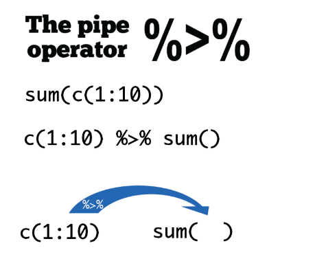
一些有用的创建功能
- 各类累计函数
cumsum(), cumprod(), cummin(), cummax(),cummean()
select()函数:根据变量的名称选择变量,选择数据框的某一列,或者某几列,或者配合一些条件选择很多列我们还是以auto数据框进行演示
select(auto,mpg) # 选auto数据框中的一个变量## # A tibble: 74 x 1
## mpg
## <dbl>
## 1 22
## 2 17
## 3 22
## 4 20
## 5 15
## 6 18
## 7 26
## 8 20
## 9 16
## 10 19
## # … with 64 more rowsselect(auto,mpg:length) # 选auto数据框中mpg列到length列的变量## # A tibble: 74 x 6
## mpg rep78 headroom trunk weight length
## <dbl> <dbl> <dbl> <dbl> <dbl> <dbl>
## 1 22 3 2.5 11 2930 186
## 2 17 3 3 11 3350 173
## 3 22 NA 3 12 2640 168
## 4 20 3 4.5 16 3250 196
## 5 15 4 4 20 4080 222
## 6 18 3 4 21 3670 218
## 7 26 NA 3 10 2230 170
## 8 20 3 2 16 3280 200
## 9 16 3 3.5 17 3880 207
## 10 19 3 3.5 13 3400 200
## # … with 64 more rowsselect(auto,-c(make,displacement))## # A tibble: 74 x 11
## price mpg rep78 headroom trunk weight length turn gear_ratio foreign w_l
## <dbl> <dbl> <dbl> <dbl> <dbl> <dbl> <dbl> <dbl> <dbl> <dbl+l> <dbl>
## 1 4099 22 3 2.5 11 2930 186 40 3.58 0 [Dom… 15.8
## 2 4749 17 3 3 11 3350 173 40 2.53 0 [Dom… 19.4
## 3 3799 22 NA 3 12 2640 168 35 3.08 0 [Dom… 15.7
## 4 4816 20 3 4.5 16 3250 196 40 2.93 0 [Dom… 16.6
## 5 7827 15 4 4 20 4080 222 43 2.41 0 [Dom… 18.4
## 6 5788 18 3 4 21 3670 218 43 2.73 0 [Dom… 16.8
## 7 4453 26 NA 3 10 2230 170 34 2.87 0 [Dom… 13.1
## 8 5189 20 3 2 16 3280 200 42 2.93 0 [Dom… 16.4
## 9 10372 16 3 3.5 17 3880 207 43 2.93 0 [Dom… 18.7
## 10 4082 19 3 3.5 13 3400 200 42 3.08 0 [Dom… 17
## # … with 64 more rowsselect(auto,contains('mp'))## # A tibble: 74 x 1
## mpg
## <dbl>
## 1 22
## 2 17
## 3 22
## 4 20
## 5 15
## 6 18
## 7 26
## 8 20
## 9 16
## 10 19
## # … with 64 more rowsrename(auto,youhao=mpg) #修改列名## # A tibble: 74 x 13
## make price youhao rep78 headroom trunk weight length turn displacement
## <chr> <dbl> <dbl> <dbl> <dbl> <dbl> <dbl> <dbl> <dbl> <dbl>
## 1 AMC … 4099 22 3 2.5 11 2930 186 40 121
## 2 AMC … 4749 17 3 3 11 3350 173 40 258
## 3 AMC … 3799 22 NA 3 12 2640 168 35 121
## 4 Buic… 4816 20 3 4.5 16 3250 196 40 196
## 5 Buic… 7827 15 4 4 20 4080 222 43 350
## 6 Buic… 5788 18 3 4 21 3670 218 43 231
## 7 Buic… 4453 26 NA 3 10 2230 170 34 304
## 8 Buic… 5189 20 3 2 16 3280 200 42 196
## 9 Buic… 10372 16 3 3.5 17 3880 207 43 231
## 10 Buic… 4082 19 3 3.5 13 3400 200 42 231
## # … with 64 more rows, and 3 more variables: gear_ratio <dbl>,
## # foreign <dbl+lbl>, w_l <dbl>除此以外还可以使用下面的命令帮助我们选择列(变量)名称
- starts_with(“abc”) 匹配以abc字符开头的列
- ends_with(“xyz”) 匹配以xyz字符结尾的列
- contains(“ijk”),匹配包含ijk字符的列
- num_range(“x”, 1:3): 匹配 x1, x2 , x3列
第一个小练习
安装nycflights13包,调入该包,调入tidyverse包,观察nycflights13包中的flights数据框。
用尽可能多的方法, 在flights中选择 dep_time, dep_delay, arr_time, and arr_delay这几列
如果你在select()调用中多次包含一个变量的名称,会发生什么?
使用mutate()对于dep_time和sched_dep_time它们不是真正的连续数字。将它们转换为更方便的表示午夜后的分钟数。
比较dep_time、sched_dep_time和dep_delay。你认为这三个数字有什么关系?
数据筛选函数filter()
- filter()允许你根据观测值进行子集。第一个参数是数据框的名称。第二个和后面的参数是过滤数据框的表达式。
比如我们选出长度大于220的汽车
dplyr:: filter(auto,length>220)## # A tibble: 5 x 13
## make price mpg rep78 headroom trunk weight length turn displacement
## <chr> <dbl> <dbl> <dbl> <dbl> <dbl> <dbl> <dbl> <dbl> <dbl>
## 1 Buic… 7827 15 4 4 20 4080 222 43 350
## 2 Cad.… 11385 14 3 4 20 4330 221 44 425
## 3 Linc… 11497 12 3 3.5 22 4840 233 51 400
## 4 Linc… 13594 12 3 2.5 18 4720 230 48 400
## 5 Merc… 5379 14 4 3.5 16 4060 221 48 302
## # … with 3 more variables: gear_ratio <dbl>, foreign <dbl+lbl>, w_l <dbl>dplyr:: filter(auto,length>220,weight>4500)## # A tibble: 2 x 13
## make price mpg rep78 headroom trunk weight length turn displacement
## <chr> <dbl> <dbl> <dbl> <dbl> <dbl> <dbl> <dbl> <dbl> <dbl>
## 1 Linc… 11497 12 3 3.5 22 4840 233 51 400
## 2 Linc… 13594 12 3 2.5 18 4720 230 48 400
## # … with 3 more variables: gear_ratio <dbl>, foreign <dbl+lbl>, w_l <dbl>比如我们可以筛选出,make里面包含“Buick”名字的汽车,结合tidyverse中的字符串处理工具,可以做很多更灵活的筛选
dplyr:: filter(auto,str_detect(make , "Buick"))## # A tibble: 7 x 13
## make price mpg rep78 headroom trunk weight length turn displacement
## <chr> <dbl> <dbl> <dbl> <dbl> <dbl> <dbl> <dbl> <dbl> <dbl>
## 1 Buic… 4816 20 3 4.5 16 3250 196 40 196
## 2 Buic… 7827 15 4 4 20 4080 222 43 350
## 3 Buic… 5788 18 3 4 21 3670 218 43 231
## 4 Buic… 4453 26 NA 3 10 2230 170 34 304
## 5 Buic… 5189 20 3 2 16 3280 200 42 196
## 6 Buic… 10372 16 3 3.5 17 3880 207 43 231
## 7 Buic… 4082 19 3 3.5 13 3400 200 42 231
## # … with 3 more variables: gear_ratio <dbl>, foreign <dbl+lbl>, w_l <dbl>dplyr:: filter(auto,str_detect(make , "AMC") | str_detect(make , "Buick") ) %>% select(make , price)## # A tibble: 10 x 2
## make price
## <chr> <dbl>
## 1 AMC Concord 4099
## 2 AMC Pacer 4749
## 3 AMC Spirit 3799
## 4 Buick Century 4816
## 5 Buick Electra 7827
## 6 Buick LeSabre 5788
## 7 Buick Opel 4453
## 8 Buick Regal 5189
## 9 Buick Riviera 10372
## 10 Buick Skylark 4082summarise()统计
- 这个函数将数据框折叠为单行,比如这样:
summarise(auto,mean_p=mean(price),na.rm=T)## # A tibble: 1 x 2
## mean_p na.rm
## <dbl> <lgl>
## 1 6165. TRUE- 如果将summarise()与group_by() 分组函数结合起来,能够发挥更好的作用,实现不同组的对比分析,例如
auto %>% group_by(foreign) %>%
  summarise(mean_w = mean(weight),mean_p=mean(price),na.rm=T)
## # A tibble: 2 x 4
## foreign mean_w mean_p na.rm
## <dbl+lbl> <dbl> <dbl> <lgl>
## 1 0 [Domestic] 3317. 6072. TRUE
## 2 1 [Foreign] 2316. 6385. TRUE可以将上面讲述的几个内容联合在一起
m <- str_split(auto$make,pattern = ' ')
make2 <- NULL
for (i in m) {
  make2 = append(make2,i[1])
}

auto %>% mutate(make2= make2) %>%
  group_by(make2) %>%
  summarise(count=n(),mean_w=mean(weight),sd_w=sd(weight),mean_p = mean(price),count=n()) %>%
  filter(mean_w>3000)
## # A tibble: 10 x 5
## make2 count mean_w sd_w mean_p
## <chr> <int> <dbl> <dbl> <dbl>
## 1 Buick 7 3399. 602. 6075.
## 2 Cad. 3 4173. 238. 13930.
## 3 Chev. 6 3063. 561. 4372.
## 4 Dodge 4 3265 766. 5056.
## 5 Linc. 3 4463. 552. 12852.
## 6 Merc. 6 3448. 641. 4914.
## 7 Olds 7 3499. 468. 6051.
## 8 Peugeot 1 3420 NA 12990
## 9 Pont. 6 3282. 344. 4879.
## 10 Volvo 1 3170 NA 11995第二个小练习
使用nycflights13包中的flights数据框。
按照dest目的地进行分组,使用n()函数计算每个目的地航班数量,平均距离,平均晚点到达时间
筛选出航班数量大于20的,且目的地不是HNL的相关数据
画出横轴(x轴)是平均距离,纵轴是平均晚点时间的散点图,谈谈二者的关系