主成分分析PCA

What —— 主成分分析的基本思想
Why —— 为什么我们需要主成分分析
一个多维特征的例子
主成分的另一种解释
How——如何进行PCA？
先做一个Scale和不Scale的对比
碎石图，选几个主成分
因子分析和主成分分析

What —— 主成分分析的基本思想

利用降维（线性变换)的思想，在损失很少信息的前提下把多个特征转化为几个不相关的综合特征（主成分),即每个主成分都是原始特征变量的线性组合,且各个主成分之间互不相关,使得主成分比原始变量具有某些更优越的性能（主成分必须保留原始特征尽可能多的信息），从而达到简化系统结构，抓住问题实质的目的。

Why —— 为什么我们需要主成分分析

假设我们的研究对象——消费者，我们拥有消费者非常全面的特征，如果要将这p个特征 $x_{1}, x_{2}, . . ., x_{p}$ 个特征可视化，实际上是相对繁琐的，人们对于太多维度的变量处理起来不够符合人类的直觉思维。

一个多维特征的例子

pacman::p_load(corrplot,DT,tidyverse,GGally,gtsummary,psych,GPArotation)

mtcars[,1:7] %>% datatable()

Show entries

Search:

	mpg	cyl	disp	hp	drat	wt	qsec
Mazda RX4	21	6	160	110	3.9	2.62	16.46
Mazda RX4 Wag	21	6	160	110	3.9	2.875	17.02
Datsun 710	22.8	4	108	93	3.85	2.32	18.61
Hornet 4 Drive	21.4	6	258	110	3.08	3.215	19.44
Hornet Sportabout	18.7	8	360	175	3.15	3.44	17.02
Valiant	18.1	6	225	105	2.76	3.46	20.22
Duster 360	14.3	8	360	245	3.21	3.57	15.84
Merc 240D	24.4	4	146.7	62	3.69	3.19	20
Merc 230	22.8	4	140.8	95	3.92	3.15	22.9
Merc 280	19.2	6	167.6	123	3.92	3.44	18.3

Showing 1 to 10 of 32 entries

Previous1 2 3 4Next

ggpairs(mtcars[,1:7]) +  theme_bw()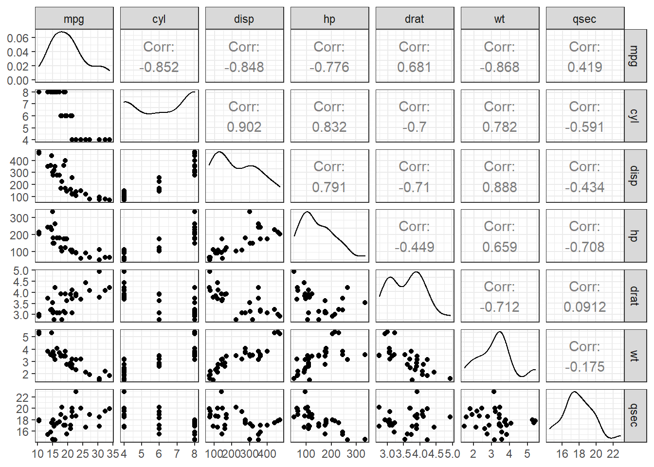

res1 <- cor.mtest(mtcars[,1:7], conf.level = .95)
corrplot(corr=cor(mtcars[,1:7]),order = "AOE",type="upper",method='pie',tl.pos = "d", p.mat = res1$p, sig.level = .1)
corrplot(corr = cor(mtcars[,1:7]),add=TRUE, type="lower", method="number",order="AOE",diag=FALSE,tl.pos="n", cl.pos="n",col="black")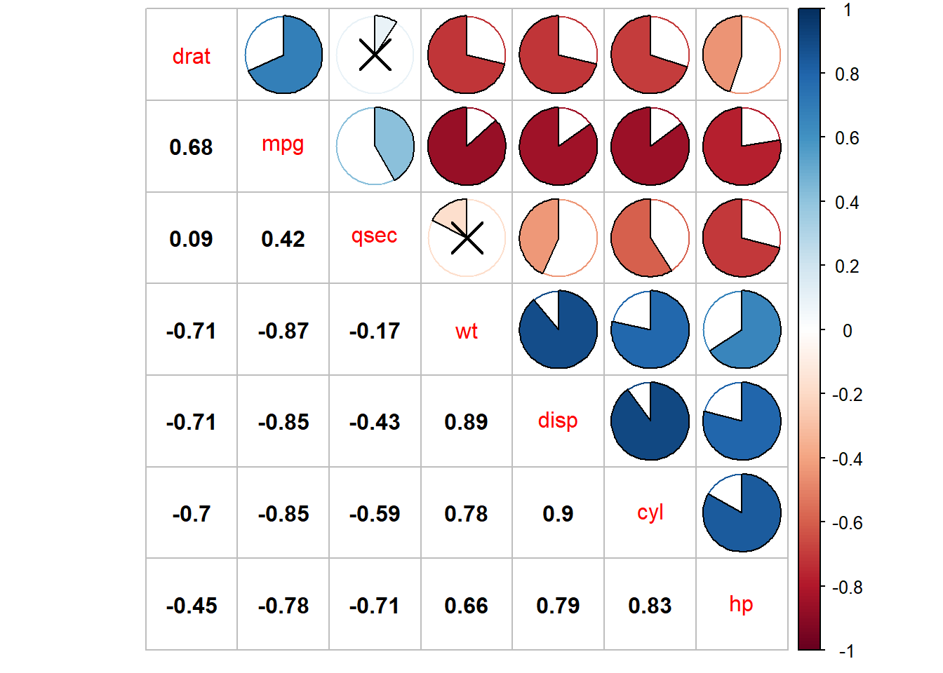

实际上这么多变量对人类进行直观分析是不友好的，虽然图画的比较漂亮，但是很可能没有图是有价值的，因为每个图或者每个特征只包含了极少的信息。很显然，如果我们研究对象的特征变得更多的时候，需要寻求一个更好的方法来可视化特征。

需要一种对数据的低纬表示，而这些表示可以尽可能多的包含特征的信息。比如，得到一个二维表示来获取数据中的大部分信息，那么就可以在这个低维空间中绘制出观测图像。

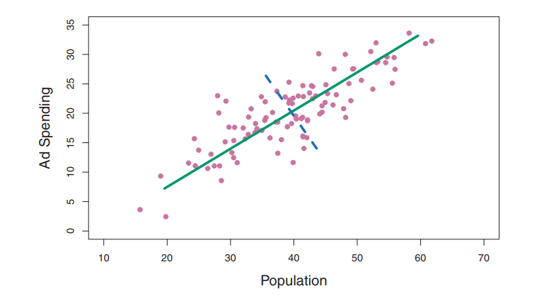
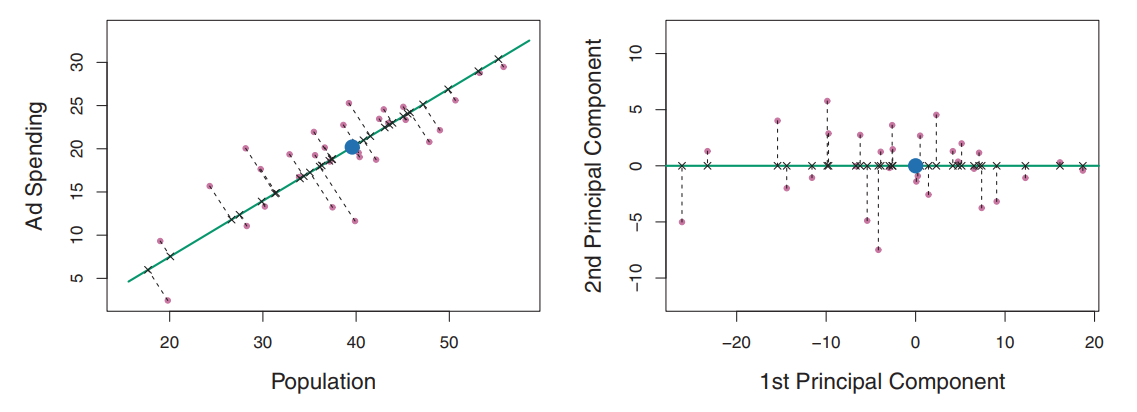
绿色实线代表数据的第一主成分方向，在这个方向上数据的波动性最大，垂直于这条线的方向的蓝色线。

$Z_{1} = 0.839 \times (p o p - \bar{p o p}) + 0.544 \times (a d - \bar{a d})$ $ϕ_{11} = 0.839, ϕ_{21} = 0.544$ 是主成分载荷，定义了主成分的方向。在满足 $ϕ_{11}^{2} + ϕ_{21}^{2} = 1$ 的约束下所有可能的pop和ad的组合里，是的这个组合的方差最大。方差大解释的变异也就越，本质上这里的目标是 $M A X : Var (ϕ_{11} \times (pop - \bar{p o p}) + ϕ_{21} \times (a d - \bar{a d}))$ 当观测值100个的时候，pop和ad也有对应的100，那么每个观测值都有一个对应的主成分： $Z_{i 1} = 0.839 \times (p o p_{i} - \bar{p o p_{i}}) + 0.544 \times (a d_{i} - \bar{a d_{i}})$

这些对应的 $z_{i 1}, z_{i 2}$ 被称为主成得分(principal component scores),下图表征了主成分得分的图例.

主成分的另一种解释

第一主成分向量定义了与数据最接近的那条线，第一主成分线使得所有点到该线的垂直距离平方和最小。第一主成分的选择使得投影得到的观测与原始观测最为接近。

主成分 $z_{i}$ 可以看作为在每个对应位置上对pop和ad数值的汇总。如果某个观测值的 $z i$ 是小于0的，表示这个观测值的两个维度ad和pop特征是低于平均水平的。那么我就做到了使用一个特征变量来指代两个特征变量的目标。

当然如果需要分析的对象有多个维度，我们还可以构造更多的主成分，目标就是使得这些主成分的方差最大，并满足不相关(垂直)条件。

How——如何进行PCA？

Scale Your Feature
Missing Value: 删除
Categorical Data

先做一个Scale和不Scale的对比

pacman::p_load(ggplot2,ggfortify)
data("USArrests")
USArrests %>% tbl_summary(statistic = list(all_continuous() ~ "均值：{mean} 方差：{sd}，最大值:{max},最小值:{min}"))

Characteristic	N = 50
Murder	均值：7.8 方差：4.4，最大值:17.4,最小值:0.8
Assault	均值：171 方差：83，最大值:337,最小值:45
UrbanPop	均值：66 方差：14，最大值:91,最小值:32
Rape	均值：21 方差：9，最大值:46,最小值:7

pr.withoutsc <- prcomp(USArrests,scale =F )
pr.withsc <- prcomp(USArrests,scale =T)

biplot(pr.withoutsc)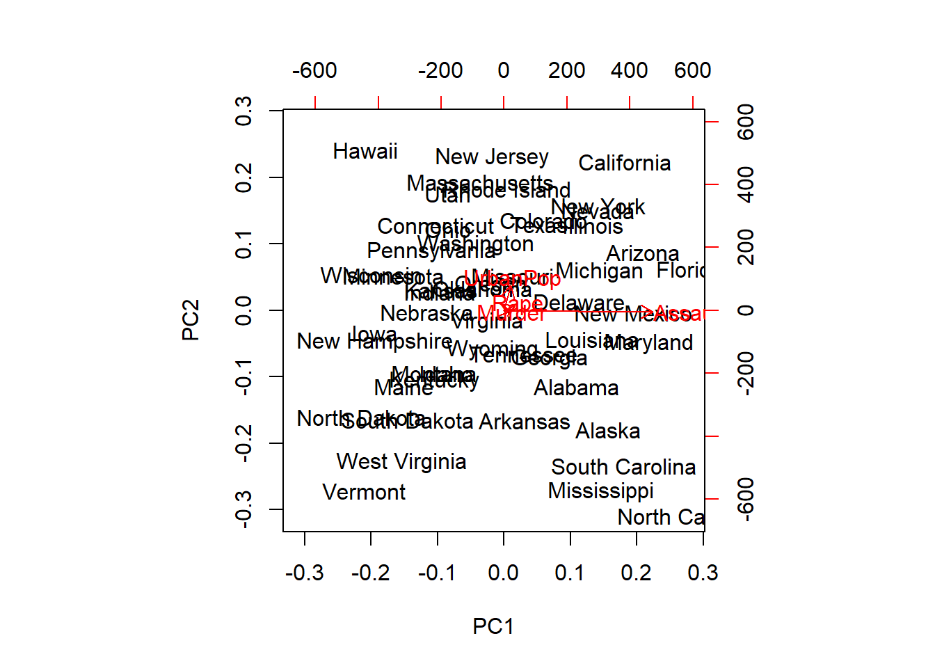

autoplot(prcomp(USArrests,scale =T),data=USArrests,label =T,loadings = TRUE,loadings.label = TRUE,loadings.label.size = 3)+
  ggthemes::theme_clean() +
  ggtitle("标准化后的主成分")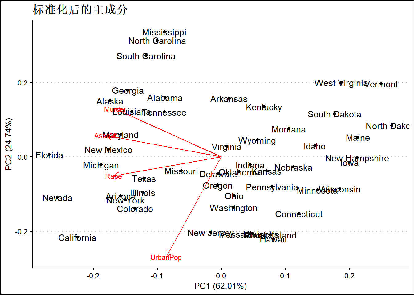

summary(pr.withsc)

## Importance of components:
##                           PC1    PC2     PC3     PC4
## Standard deviation     1.5749 0.9949 0.59713 0.41645
## Proportion of Variance 0.6201 0.2474 0.08914 0.04336
## Cumulative Proportion  0.6201 0.8675 0.95664 1.00000

#rotation矩阵提供了主成分的载荷信息
pr.withsc$rotation

##                 PC1        PC2        PC3         PC4
## Murder   -0.5358995  0.4181809 -0.3412327  0.64922780
## Assault  -0.5831836  0.1879856 -0.2681484 -0.74340748
## UrbanPop -0.2781909 -0.8728062 -0.3780158  0.13387773
## Rape     -0.5434321 -0.1673186  0.8177779  0.08902432

如果希望观察每个观测值或者说周的某个主成分得分比如PC1第一个主成分得分

head(pr.withsc$x)

##                   PC1        PC2         PC3          PC4
## Alabama    -0.9756604  1.1220012 -0.43980366  0.154696581
## Alaska     -1.9305379  1.0624269  2.01950027 -0.434175454
## Arizona    -1.7454429 -0.7384595  0.05423025 -0.826264240
## Arkansas    0.1399989  1.1085423  0.11342217 -0.180973554
## California -2.4986128 -1.5274267  0.59254100 -0.338559240
## Colorado   -1.4993407 -0.9776297  1.08400162  0.001450164

as.data.frame(pr.withsc$x) %>% select(PC1,PC2) %>% datatable()

Show entries

Search:

	PC1	PC2
Alabama	-0.975660448333605	1.12200121043341
Alaska	-1.93053787851368	1.06242691953445
Arizona	-1.7454428533906	-0.738459537284998
Arkansas	0.139998944348595	1.10854225950591
California	-2.49861284825858	-1.52742672082479
Colorado	-1.49934073746552	-0.977629656524983
Connecticut	1.34499236494685	-1.07798361522603
Delaware	-0.0472298063468948	-0.322088902660565
Florida	-2.98275966985053	0.0388342468594005
Georgia	-1.62280741822275	1.26608838405527

Showing 1 to 10 of 50 entries

Previous1 2 3 4 5Next

碎石图，选几个主成分

接下来画一个碎石图，观察主成分个数增加对特征向量解释力度的变化

pr.var <- (pr.withsc$sdev)^2
pve <- pr.var / sum(pr.var)
df <- tibble(x=seq(1,4,by=1),y=pve)
ggplot(df,aes(x=x,y=y))+
  geom_point()+geom_line() +theme_bw() +ggtitle("碎石图")+
  xlab('主成分个数') + ylab('每个主成分解释的变异')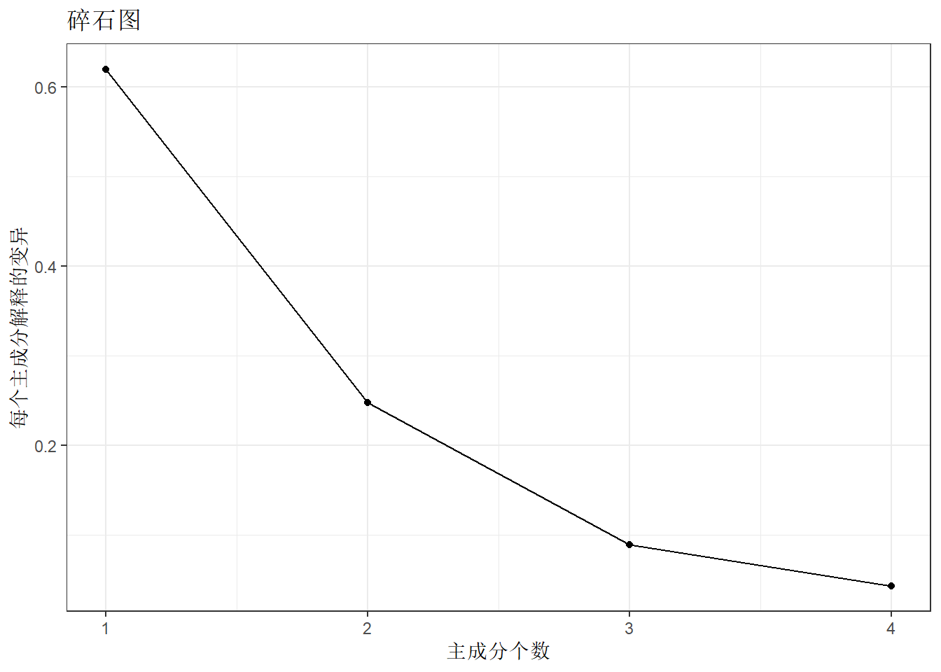

fa.parallel(cor(USArrests), n.obs=112, fa='both', n.iter=100)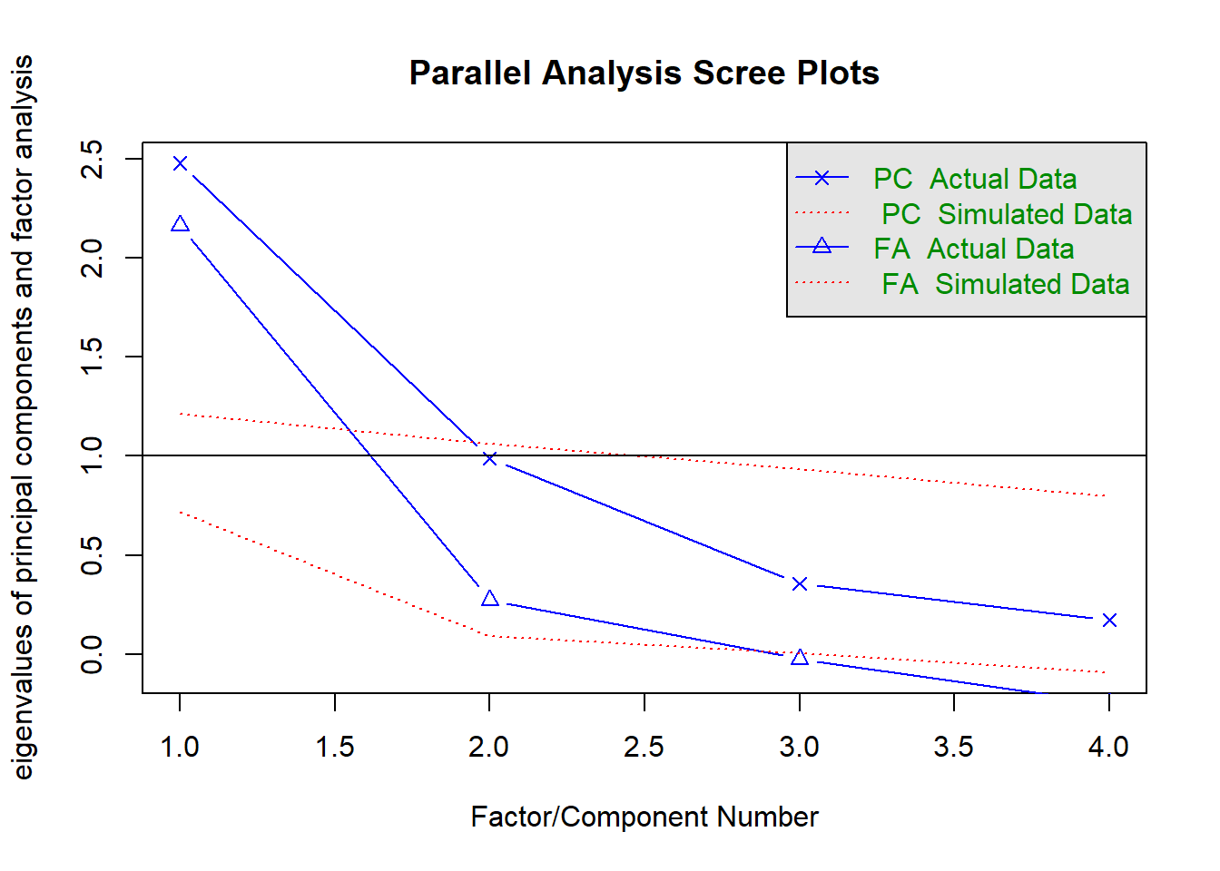

## Parallel analysis suggests that the number of factors =  2  and the number of components =  1

dim(USArrests)

## [1] 50  4

通常可以通过看碎石图来决定所需的主成分数量。我们选择满足要求的最少数量的主成分来解释数据中的绝大部分变异。

通过观察碎石图，可以找到一个点，在这个点上，主成分解释的方差比例突然减少。

这个点就被视为肘(elbow),选择肘出现的个数作为主成分分析的个数。

这种可视化分析感觉有些随意。遗憾的是，没有一个被广泛认可的客观方法来决定多少主成分才够用。事实上，多少个主成分才够用这个提法就比较欠妥，这个问题取决于特定的应用领域和特定的数据集。

在实践中，往往通过看前几个主成分来寻找数据中有价值的模式。如果在前几个主成分中都找不到有价值的模式，那更多的主成分也不太可能会有价值。相反，如果前几个主成分有价值，那通常会继续观察随后的主成分，直到找不到更多有价值的模式为止。

因子分析和主成分分析

主成分分析就是你有一堆的特征变量X1,X2,x3,….它们可以通过添加不同的权重组合成一些个主成分F1，F2，F3….，可以理解为观测变量是因，主成分是果。

因子分析就是你有一堆的观测变量X1，X2，X3….，同时你有一些个未知的因子F1，F2，F3…，这些因子可以通过添加不同的权重组合成那些个观测变量，可以理解为因子是因，观测变量是果。

因子分析仅举个例子，不展开讲细节

data(bfi)
bfi <- bfi[,1:23]
bfi <- drop_na(bfi)
corrplot(corr=cor(bfi[,1:7]),order = "AOE",type="upper",method='pie',tl.pos = "d", p.mat = res1$p, sig.level = .1)
corrplot(corr = cor(bfi[,1:7]),add=TRUE, type="lower", method="number",order="AOE",diag=FALSE,tl.pos="n", cl.pos="n",col="black")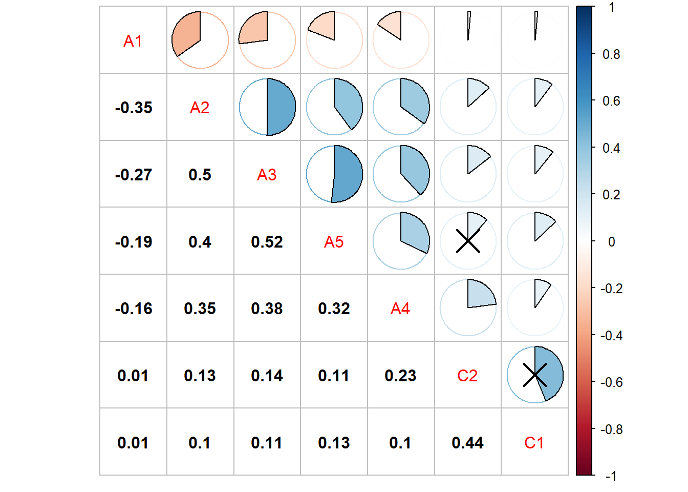

fa.parallel(cor(bfi), n.obs=112, fa="fa", n.iter=100)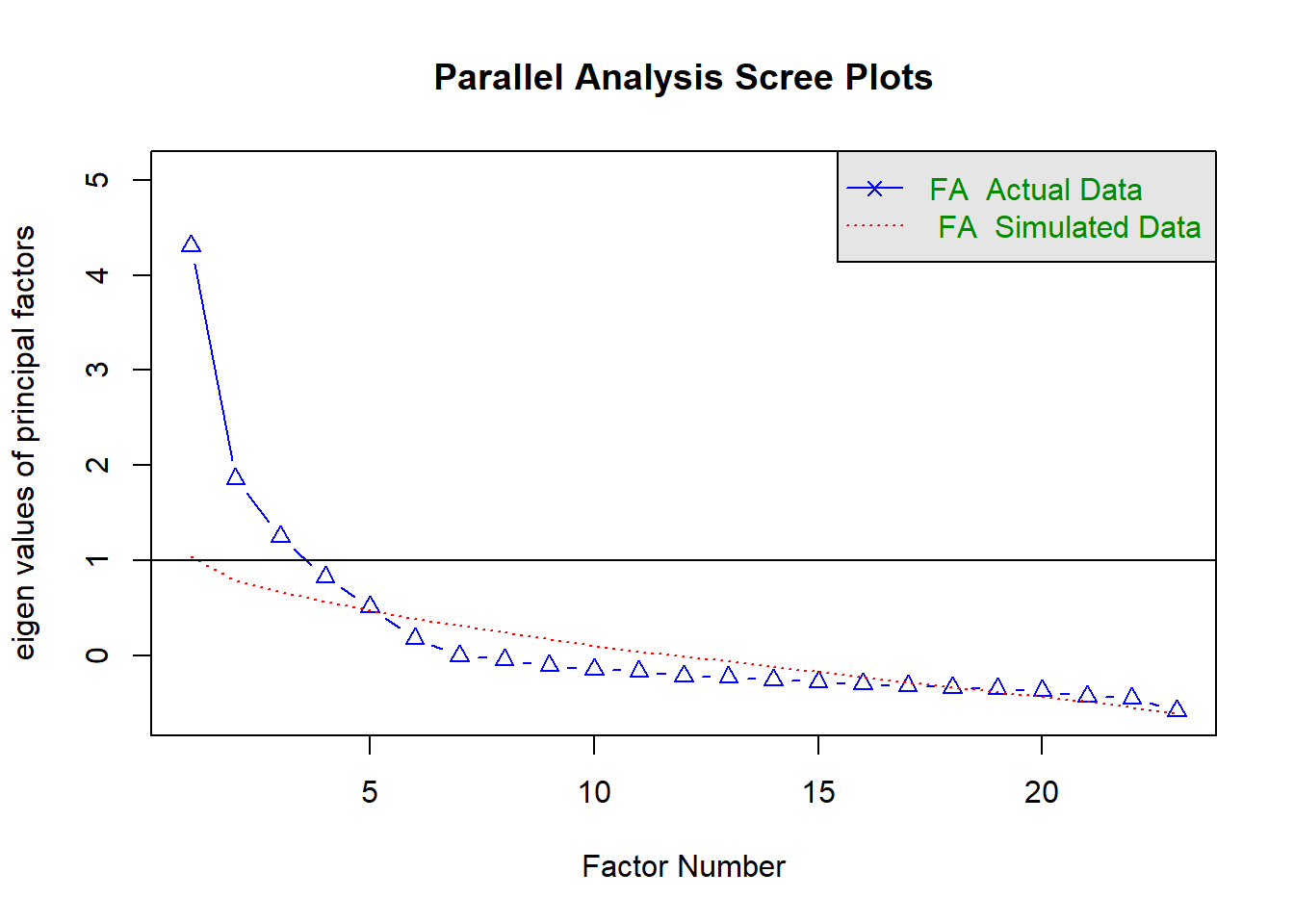

## Parallel analysis suggests that the number of factors =  5  and the number of components =  NA

# 建议我们选5个公因子，那就选5个
fa_model <- fa(cor(bfi),nfactors = 5,rotate = 'none',fm='pa')
fa_model

## Factor Analysis using method =  pa
## Call: fa(r = cor(bfi), nfactors = 5, rotate = "none", fm = "pa")
## Standardized loadings (pattern matrix) based upon correlation matrix
##      PA1   PA2   PA3   PA4   PA5   h2   u2 com
## A1 -0.22  0.00  0.15 -0.25 -0.21 0.18 0.82 3.6
## A2  0.47  0.28 -0.14  0.34  0.16 0.46 0.54 3.1
## A3  0.54  0.31 -0.22  0.29  0.18 0.55 0.45 2.9
## A4  0.42  0.13 -0.03  0.33  0.00 0.30 0.70 2.1
## A5  0.59  0.18 -0.24  0.16  0.10 0.47 0.53 1.8
## C1  0.34  0.11  0.47 -0.03  0.03 0.35 0.65 2.0
## C2  0.33  0.19  0.55  0.11  0.03 0.46 0.54 2.0
## C3  0.32  0.05  0.43  0.17 -0.05 0.32 0.68 2.3
## C4 -0.46  0.12 -0.49 -0.09  0.09 0.48 0.52 2.3
## C5 -0.49  0.14 -0.36 -0.10  0.17 0.43 0.57 2.4
## E1 -0.41 -0.20  0.27  0.17  0.24 0.36 0.64 3.4
## E2 -0.62 -0.06  0.21  0.18  0.29 0.55 0.45 1.9
## E3  0.53  0.32 -0.15 -0.21  0.06 0.45 0.55 2.2
## E4  0.61  0.19 -0.26  0.01 -0.24 0.53 0.47 1.9
## E5  0.51  0.29  0.11 -0.19 -0.12 0.41 0.59 2.2
## N1 -0.44  0.65  0.09 -0.07 -0.23 0.68 0.32 2.1
## N2 -0.42  0.63  0.12 -0.07 -0.17 0.62 0.38 2.1
## N3 -0.40  0.61  0.06  0.03  0.00 0.54 0.46 1.8
## N4 -0.53  0.40  0.06  0.07  0.26 0.52 0.48 2.4
## N5 -0.34  0.42  0.04  0.23  0.02 0.35 0.65 2.6
## O1  0.32  0.18  0.09 -0.36  0.28 0.35 0.65 3.6
## O2 -0.18  0.10 -0.16  0.30 -0.23 0.21 0.79 3.5
## O3  0.40  0.27  0.03 -0.41  0.32 0.50 0.50 3.7
## 
##                        PA1  PA2  PA3  PA4  PA5
## SS loadings           4.55 2.22 1.50 1.04 0.75
## Proportion Var        0.20 0.10 0.07 0.05 0.03
## Cumulative Var        0.20 0.29 0.36 0.40 0.44
## Proportion Explained  0.45 0.22 0.15 0.10 0.07
## Cumulative Proportion 0.45 0.67 0.82 0.93 1.00
## 
## Mean item complexity =  2.5
## Test of the hypothesis that 5 factors are sufficient.
## 
## The degrees of freedom for the null model are  253  and the objective function was  7.03
## The degrees of freedom for the model are 148  and the objective function was  0.54 
## 
## The root mean square of the residuals (RMSR) is  0.03 
## The df corrected root mean square of the residuals is  0.04 
## 
## Fit based upon off diagonal values = 0.98
## Measures of factor score adequacy             
##                                                    PA1  PA2  PA3  PA4  PA5
## Correlation of (regression) scores with factors   0.95 0.91 0.85 0.80 0.77
## Multiple R square of scores with factors          0.90 0.83 0.73 0.64 0.59
## Minimum correlation of possible factor scores     0.80 0.67 0.45 0.28 0.19

结果显示，五个因子解释了原始23个变量的44%的方差，有点低啊

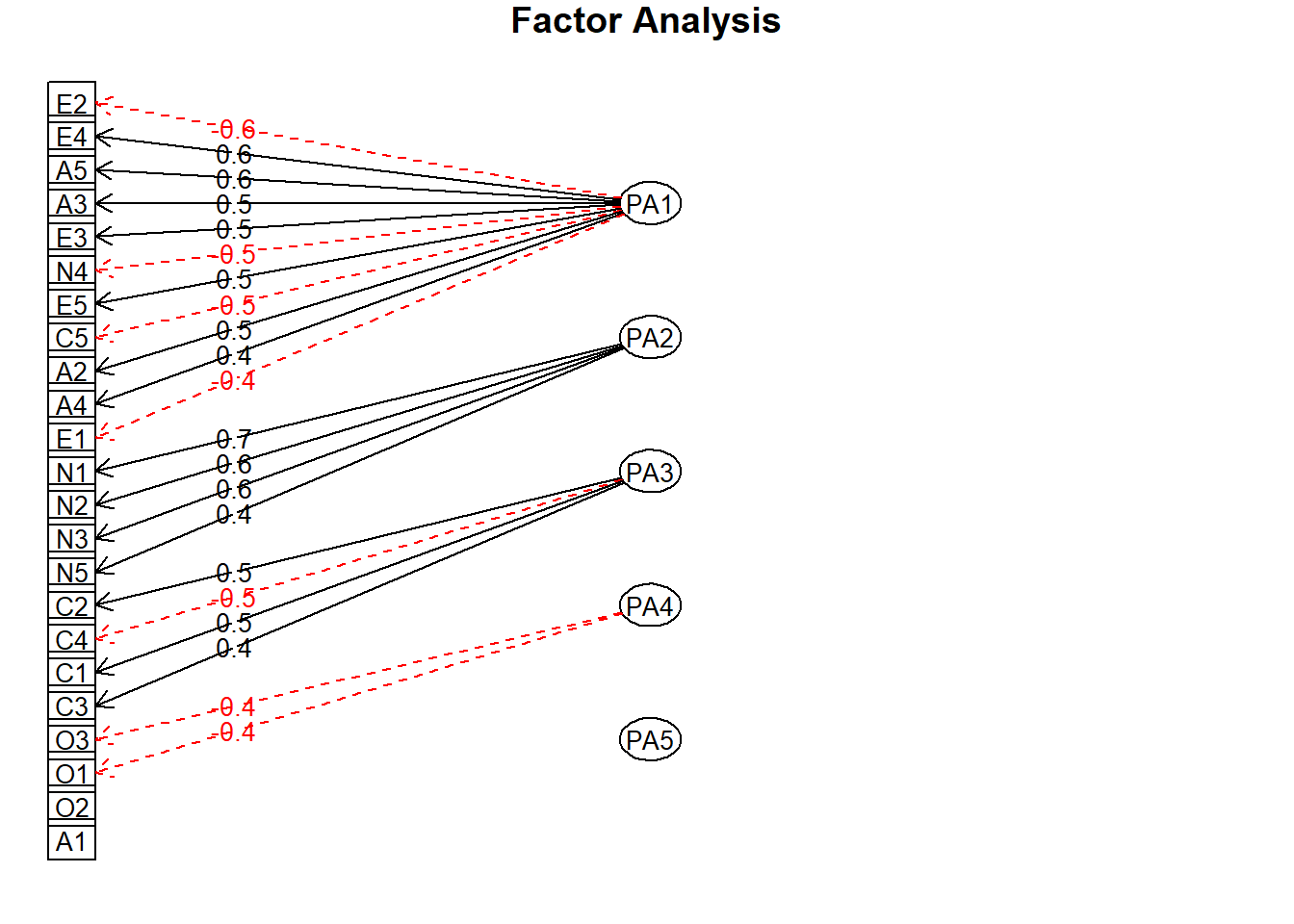
整个因子分析的结构图如下

fa.diagram(fa_model)

张剑

2020/03/25

What —— 主成分分析的基本思想

Why —— 为什么我们需要主成分分析

一个多维特征的例子

需要一种对数据的低纬表示，而这些表示可以尽可能多的包含特征的信息。比如，得到一个二维表示来获取数据中的大部分信息，那么就可以在这个低维空间中绘制出观测图像。

绿色实线代表数据的第一主成分方向，在这个方向上数据的波动性最大，垂直于这条线的方向的蓝色线。

这些对应的 $z_{i 1}, z_{i 2}$ 被称为主成得分(principal component scores),下图表征了主成分得分的图例.

主成分的另一种解释

主成分 $z_{i}$ 可以看作为在每个对应位置上对pop和ad数值的汇总。如果某个观测值的 $z i$ 是小于0的，表示这个观测值的两个维度ad和pop特征是低于平均水平的。那么我就做到了使用一个特征变量来指代两个特征变量的目标。

How——如何进行PCA？

先做一个Scale和不Scale的对比

如果希望观察每个观测值或者说周的某个主成分得分比如PC1第一个主成分得分

碎石图，选几个主成分

接下来画一个碎石图，观察主成分个数增加对特征向量解释力度的变化

通常可以通过看碎石图来决定所需的主成分数量。我们选择满足要求的最少数量的主成分来解释数据中的绝大部分变异。

通过观察碎石图，可以找到一个点，在这个点上，主成分解释的方差比例突然减少。

这个点就被视为肘(elbow),选择肘出现的个数作为主成分分析的个数。

因子分析和主成分分析

主成分分析就是你有一堆的特征变量X1,X2,x3,….它们可以通过添加不同的权重组合成一些个主成分F1，F2，F3….，可以理解为观测变量是因，主成分是果。

因子分析就是你有一堆的观测变量X1，X2，X3….，同时你有一些个未知的因子F1，F2，F3…，这些因子可以通过添加不同的权重组合成那些个观测变量，可以理解为因子是因，观测变量是果。

因子分析仅举个例子，不展开讲细节

结果显示，五个因子解释了原始23个变量的44%的方差，有点低啊

整个因子分析的结构图如下

主成分分析PCA

张剑

2020/03/25

What —— 主成分分析的基本思想

Why —— 为什么我们需要主成分分析

一个多维特征的例子

需要一种对数据的低纬表示，而这些表示可以尽可能多的包含特征的信息。比如，得到一个二维表示来获取数据中的大部分信息，那么就可以在这个低维空间中绘制出观测图像。

绿色实线代表数据的第一主成分方向，在这个方向上数据的波动性最大，垂直于这条线的方向的蓝色线。

这些对应的zi1,zi2zi1,zi2被称为主成得分(principal component scores),下图表征了主成分得分的图例.

主成分的另一种解释

主成分zizi可以看作为在每个对应位置上对pop和ad数值的汇总。如果某个观测值的zizi是小于0的，表示这个观测值的两个维度ad和pop特征是低于平均水平的。那么我就做到了使用一个特征变量来指代两个特征变量的目标。

How——如何进行PCA？

先做一个Scale和不Scale的对比

如果希望观察每个观测值或者说周的某个主成分得分比如PC1第一个主成分得分

碎石图，选几个主成分

接下来画一个碎石图，观察主成分个数增加对特征向量解释力度的变化

通常可以通过看碎石图来决定所需的主成分数量。我们选择满足要求的最少数量的主成分来解释数据中的绝大部分变异。

通过观察碎石图，可以找到一个点，在这个点上，主成分解释的方差比例突然减少。

这个点就被视为肘(elbow),选择肘出现的个数作为主成分分析的个数。

因子分析和主成分分析

主成分分析就是你有一堆的特征变量X1,X2,x3,….它们可以通过添加不同的权重组合成一些个主成分F1，F2，F3….，可以理解为观测变量是因，主成分是果。

因子分析就是你有一堆的观测变量X1，X2，X3….，同时你有一些个未知的因子F1，F2，F3…，这些因子可以通过添加不同的权重组合成那些个观测变量，可以理解为因子是因，观测变量是果。

因子分析仅举个例子，不展开讲细节

结果显示，五个因子解释了原始23个变量的44%的方差，有点低啊

整个因子分析的结构图如下

这些对应的 $z_{i 1}, z_{i 2}$ 被称为主成得分(principal component scores),下图表征了主成分得分的图例.

主成分 $z_{i}$ 可以看作为在每个对应位置上对pop和ad数值的汇总。如果某个观测值的 $z i$ 是小于0的，表示这个观测值的两个维度ad和pop特征是低于平均水平的。那么我就做到了使用一个特征变量来指代两个特征变量的目标。