Interrupted Time-series Analysis(ITSA) 中断时间序列分析
当只有一个研究组(无对照组)时,标准ITSA回归模型采用以下形式
数据链接
\[Y_{t}=\beta_{0}+\beta_{1} T_{t}+\beta_{2} X_{t}+\beta_{3} X_{t} T_{t}+\epsilon_{t}\]
- 其中\(Y_t\)为每个等距时间点t上测量的结果变量
- \(T_t\)是从研究开始的时间趋势
- \(X_t\)是一个虚拟变量去衡量政策干预(intervention)(干预之前为0,干预之后为1)
- \(X_tT_t\)是交互项,用来表示干预后的趋势 我们在这里假设模型服从AR(1)
我们使用1988 California Proposition 99,烟草税与健康保护法为例,先实现ITSA方法以及使用谷歌开发的CausalImpact测试Bayesian structural time-series models
调包侠开始表演
library(tidyverse)
library(sandwich)
library(stargazer)
library(lmtest)
library(ggthemes)
cig <- read_csv("~/jefeerzhang/content/post/data/cigsales_2.csv") #提前设置工作目录
head(cig)
## # A tibble: 6 x 15
## uid year state cigsale lnincome beer age15to24 retprice time california
## <dbl> <dbl> <chr> <dbl> <dbl> <dbl> <dbl> <dbl> <dbl> <dbl>
## 1 1 1970 Alab… 89.8 NA NA 0.179 39.6 0 0
## 2 2 1971 Alab… 95.4 NA NA 0.180 42.7 1 0
## 3 3 1972 Alab… 101. 9.50 NA 0.181 42.3 2 0
## 4 4 1973 Alab… 103. 9.55 NA 0.182 42.1 3 0
## 5 5 1974 Alab… 108. 9.54 NA 0.183 43.1 4 0
## 6 6 1975 Alab… 112. 9.54 NA 0.184 46.6 5 0
## # … with 5 more variables: cal_trend <dbl>, tax_dummy <dbl>, tax_trend <dbl>,
## # cal_tax_dummy <dbl>, cal_tax_trend <dbl>names(cig)## [1] "uid" "year" "state" "cigsale"
## [5] "lnincome" "beer" "age15to24" "retprice"
## [9] "time" "california" "cal_trend" "tax_dummy"
## [13] "tax_trend" "cal_tax_dummy" "cal_tax_trend"cig_c <- cig %>%
filter(state == "California")
mod1 <- lm(cigsale ~ time + tax_dummy + tax_trend,data=cig_c)
stargazer(mod1,type = 'text')##
## ===============================================
## Dependent variable:
## ---------------------------
## cigsale
## -----------------------------------------------
## time -1.779***
## (0.217)
##
## tax_dummy -20.058***
## (3.747)
##
## tax_trend -1.495***
## (0.485)
##
## Constant 132.226***
## (2.287)
##
## -----------------------------------------------
## Observations 31
## R2 0.973
## Adjusted R2 0.970
## Residual Std. Error 5.182 (df = 27)
## F Statistic 326.359*** (df = 3; 27)
## ===============================================
## Note: *p<0.1; **p<0.05; ***p<0.01coeftest(mod1,vcov=NeweyWest(mod1,lag = 1, prewhite = 0,adjust = T))##
## t test of coefficients:
##
## Estimate Std. Error t value Pr(>|t|)
## (Intercept) 132.22579 4.25305 31.0896 < 2.2e-16 ***
## time -1.77947 0.38342 -4.6411 7.991e-05 ***
## tax_dummy -20.05810 4.72440 -4.2456 0.0002304 ***
## tax_trend -1.49465 0.43682 -3.4217 0.0019968 **
## ---
## Signif. codes: 0 '***' 0.001 '**' 0.01 '*' 0.05 '.' 0.1 ' ' 1ggplot(cig_c,aes(x=year,y=cigsale)) +
geom_point(size=1.4)+
geom_smooth(data=subset(cig_c,year<=1989),method = 'lm',se=F)+
geom_smooth(data=subset(cig_c,year>1989),method = 'lm',se=F)+
geom_vline(xintercept = 1989,linetype='dashed') + theme_calc()+
labs(title = "1989年加州烟草税对香烟销量的影响")+
theme(text = element_text(family='Kai'))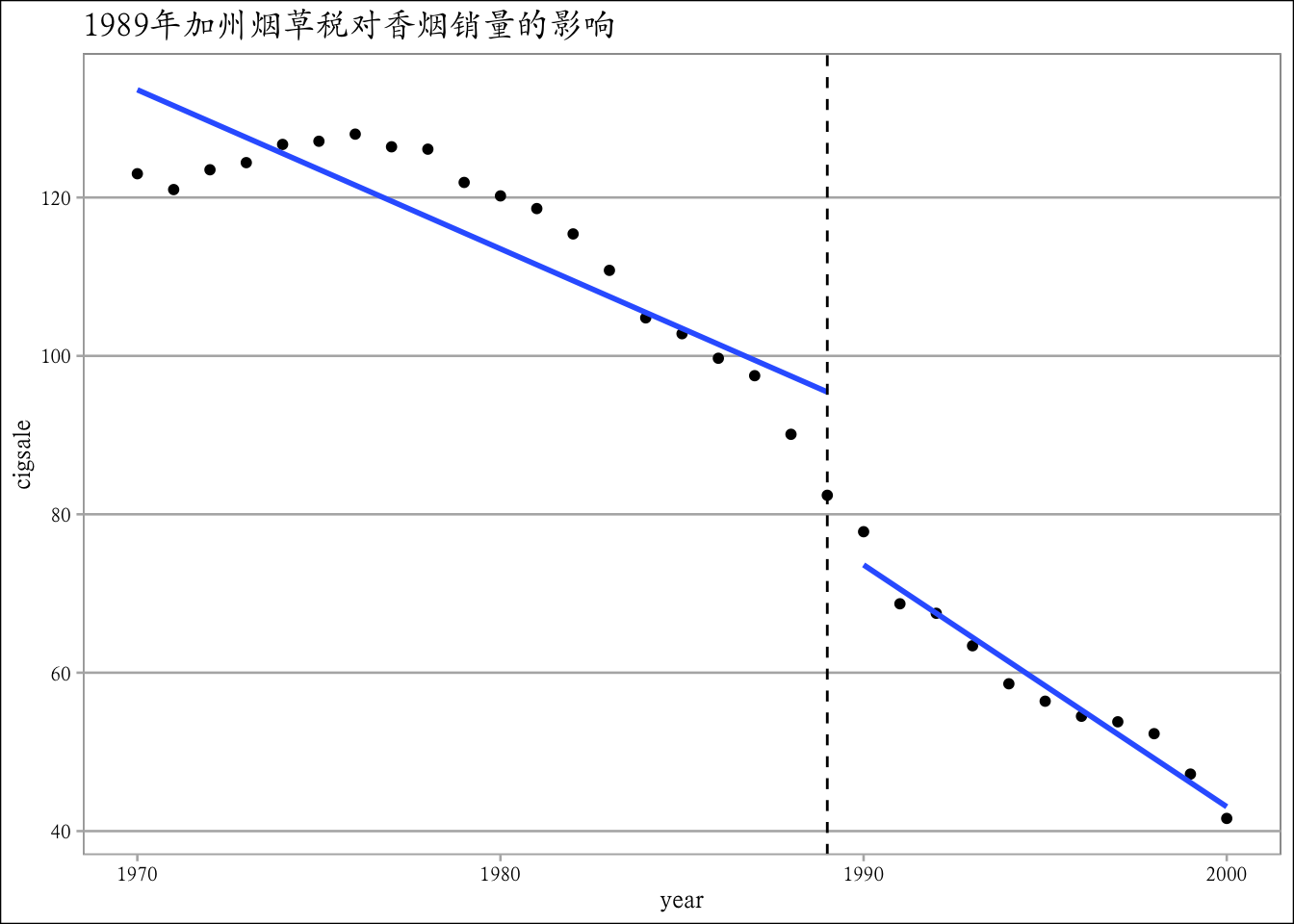
接下来使用CausalImpact进行测试
library(CausalImpact)## 载入需要的程辑包:bsts## 载入需要的程辑包:BoomSpikeSlab## 载入需要的程辑包:Boom## 载入需要的程辑包:MASS##
## 载入程辑包:'MASS'## The following object is masked from 'package:dplyr':
##
## select##
## 载入程辑包:'Boom'## The following object is masked from 'package:stats':
##
## rWishart##
## 载入程辑包:'BoomSpikeSlab'## The following object is masked from 'package:stats':
##
## knots## 载入需要的程辑包:xts##
## 载入程辑包:'xts'## The following objects are masked from 'package:dplyr':
##
## first, last##
## 载入程辑包:'bsts'## The following object is masked from 'package:BoomSpikeSlab':
##
## SuggestBurnlibrary(tidyverse)
library(zoo)
library(anytime)
cig_c_Cas <- cig_c %>% dplyr::select(cigsale,time)
pre.period <- c(0, 19)
post.period <- c(20, 30)
impact <- CausalImpact(cig_c_Cas, pre.period ,post.period)## Warning in FormatInputPrePostPeriod(pre.period, post.period, data): Setting
## pre.period[1] to start of data: 1plot(impact)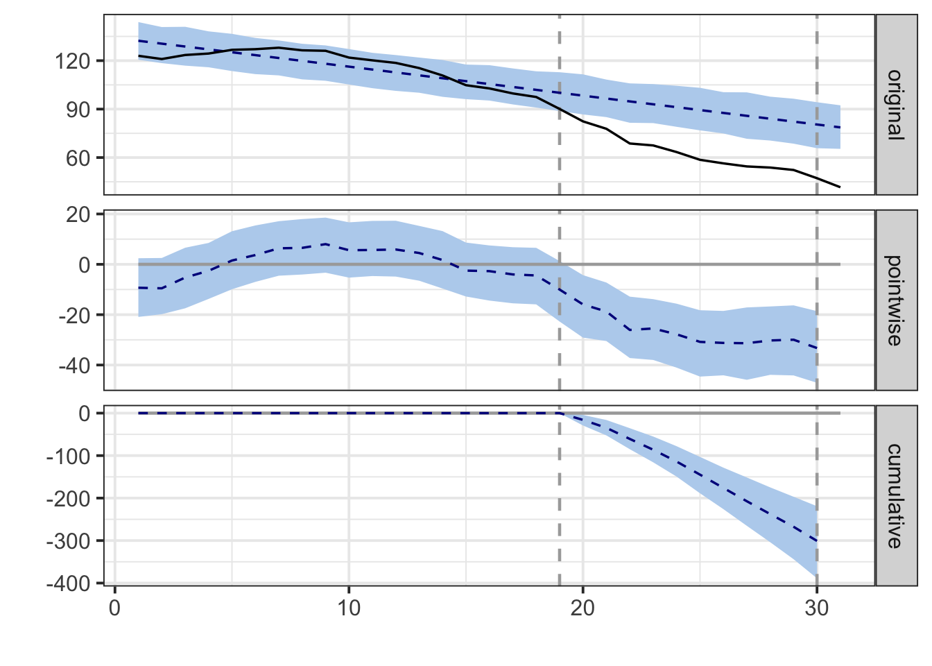
summary(impact)## Posterior inference {CausalImpact}
##
## Average Cumulative
## Actual 62 683
## Prediction (s.d.) 89 (3.9) 983 (43.3)
## 95% CI [82, 97] [902, 1071]
##
## Absolute effect (s.d.) -27 (3.9) -301 (43.3)
## 95% CI [-35, -20] [-389, -219]
##
## Relative effect (s.d.) -31% (4.4%) -31% (4.4%)
## 95% CI [-40%, -22%] [-40%, -22%]
##
## Posterior tail-area probability p: 0.00102
## Posterior prob. of a causal effect: 99.89775%
##
## For more details, type: summary(impact, "report")使用其他非加州的地区作为控制组,将加州作为控制组,使用如下模型
\[Y_{t}=\beta_{0}+\beta_{1} T_{t}+\beta_{2} X_{t}+\beta_{3} X_{t} T_{t}+\beta_{4} Z+\beta_{5} Z T_{t}+\beta_{6} Z X_{t}+\beta_{7} Z X_{t} T_{t}+\epsilon_{t}\] 其中:
Z为虚拟变量,加州为1,控制州为0
\(ZT_T\)和\(Z_tT_t\)和\(ZX_tT_t\)为虚拟变量与其他变量的交互项
图示如下
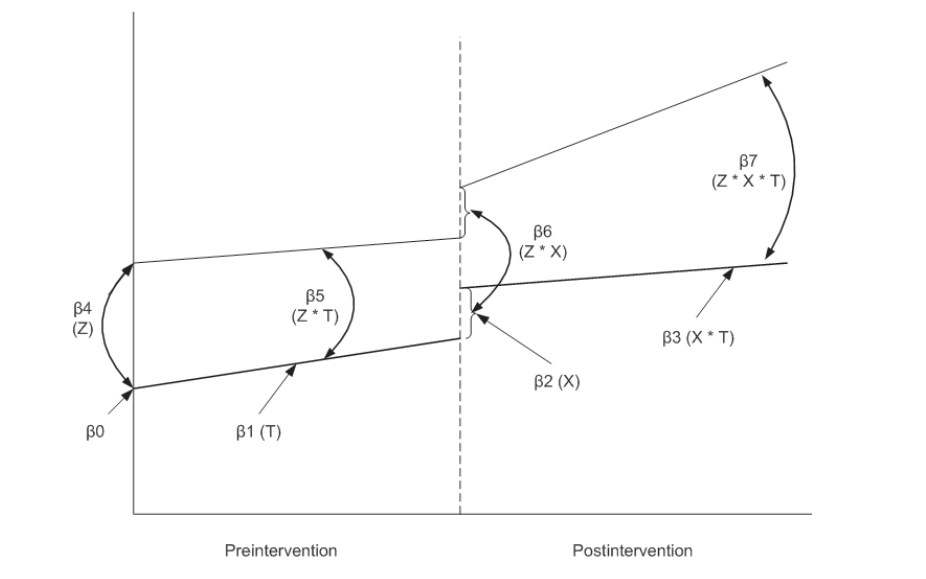
- \(\beta_0\)和\(\beta_3\)代表了控制组
- \(\beta_4\)和\(\beta_7\)代表了处理组
- \(\beta_4\)代表了控制组与处理组在干预(政策)之前的差异
- \(\beta_5\)代表了干预之后的差异
- \(\beta_6\)反应了当干预发生时(即刻)处理组和控制组的差异
- \(\beta_7\)反应了干预之后处理组和控制组之间的差异 我们在这里同样假设模型服从AR(1)
mod2 <- lm(cigsale ~ time + california +cal_trend +tax_trend + tax_dummy + cal_tax_dummy +
             cal_tax_trend,data=cig)
stargazer(mod2,type = 'text')
##
## ===============================================
## Dependent variable:
## ---------------------------
## cigsale
## -----------------------------------------------
## time -0.548***
## (0.197)
##
## california -3.274
## (12.979)
##
## cal_trend -1.232
## (1.232)
##
## tax_trend -0.504
## (0.440)
##
## tax_dummy -17.252***
## (3.406)
##
## cal_tax_dummy -2.806
## (21.269)
##
## cal_tax_trend -0.991
## (2.751)
##
## Constant 135.499***
## (2.078)
##
## -----------------------------------------------
## Observations 1,209
## R2 0.220
## Adjusted R2 0.215
## Residual Std. Error 29.032 (df = 1201)
## F Statistic 48.269*** (df = 7; 1201)
## ===============================================
## Note: *p<0.1; **p<0.05; ***p<0.01coeftest(mod2,vcov = NeweyWest(mod2,lag =1 ,prewhite = 0,adjust=T) )##
## t test of coefficients:
##
## Estimate Std. Error t value Pr(>|t|)
## (Intercept) 135.49946 3.55391 38.1268 < 2.2e-16 ***
## time -0.54777 0.29413 -1.8623 0.062798 .
## california -3.27367 5.33758 -0.6133 0.539778
## cal_trend -1.23170 0.46412 -2.6539 0.008063 **
## tax_trend -0.50351 0.52350 -0.9618 0.336339
## tax_dummy -17.25168 3.82091 -4.5151 6.952e-06 ***
## cal_tax_dummy -2.80642 5.84476 -0.4802 0.631202
## cal_tax_trend -0.99114 0.66460 -1.4913 0.136133
## ---
## Signif. codes: 0 '***' 0.001 '**' 0.01 '*' 0.05 '.' 0.1 ' ' 1# 作图
# 先把数据整合一下,处理组一个均值,当然处理组就一个,控制组一个均值,控制组有很多
aggdata <- aggregate(cig,by=list(cig$california,cig$year), FUN = mean,na.rm=T)
str(aggdata)## 'data.frame': 62 obs. of 17 variables:
## $ Group.1 : num 0 1 0 1 0 1 0 1 0 1 ...
## $ Group.2 : num 1970 1970 1971 1971 1972 ...
## $ uid : num 604 63 605 64 606 ...
## $ year : num 1970 1970 1971 1971 1972 ...
## $ state : num NA NA NA NA NA NA NA NA NA NA ...
## $ cigsale : num 120 123 124 121 129 ...
## $ lnincome : num NaN NaN NaN NaN 9.68 ...
## $ beer : num NaN NaN NaN NaN NaN NaN NaN NaN NaN NaN ...
## $ age15to24 : num 0.178 0.178 0.179 0.179 0.181 ...
## $ retprice : num 35.9 38.8 37.9 39.7 39.3 ...
## $ time : num 0 0 1 1 2 2 3 3 4 4 ...
## $ california : num 0 1 0 1 0 1 0 1 0 1 ...
## $ cal_trend : num 0 0 0 1 0 2 0 3 0 4 ...
## $ tax_dummy : num 0 0 0 0 0 0 0 0 0 0 ...
## $ tax_trend : num 0 0 0 0 0 0 0 0 0 0 ...
## $ cal_tax_dummy: num 0 0 0 0 0 0 0 0 0 0 ...
## $ cal_tax_trend: num 0 0 0 0 0 0 0 0 0 0 ...table(aggdata$Group.1)##
## 0 1
## 31 31ggplot(aggdata,aes(x=Group.2,y=cigsale,color=as.factor(Group.1 ))) +
geom_point(size=1.5)+geom_vline(xintercept = 1989,linetype='dashed') +theme_clean()+
geom_smooth(data = subset(aggdata,Group.2 <= 1989), method = "lm",se=F)+
geom_smooth(data = subset(aggdata,Group.2 > 1989), method = "lm",se=F) +
ggtitle('1989年加州香烟法令对销量的影响') + xlab('年份') + ylab("香烟销量")+
theme(text = element_text(family='Kai'))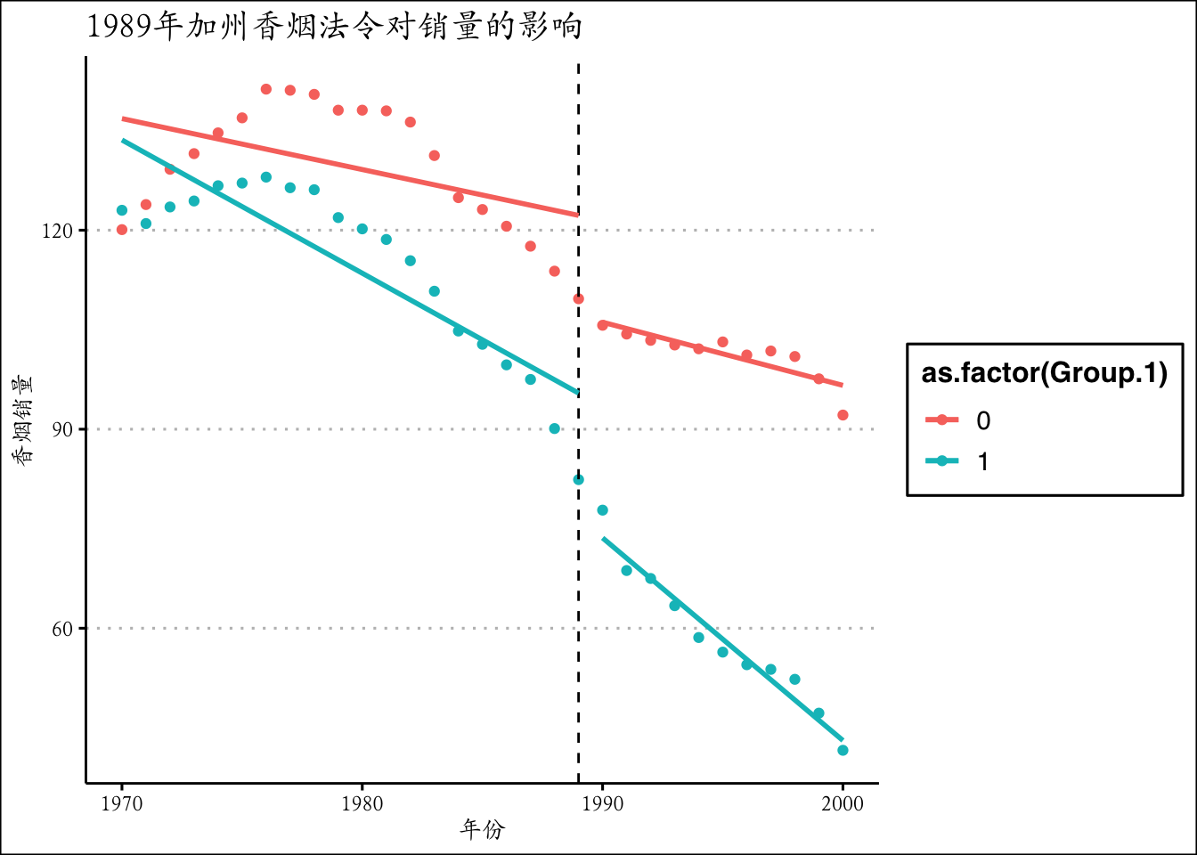
接下来继续使用CausalImpact进行测试,在其中加入其他州的均值作为解释变量
library(CausalImpact)
library(tidyverse)
library(zoo)
library(anytime)
str(aggdata)
## 'data.frame': 62 obs. of 17 variables:
## $ Group.1 : num 0 1 0 1 0 1 0 1 0 1 ...
## $ Group.2 : num 1970 1970 1971 1971 1972 ...
## $ uid : num 604 63 605 64 606 ...
## $ year : num 1970 1970 1971 1971 1972 ...
## $ state : num NA NA NA NA NA NA NA NA NA NA ...
## $ cigsale : num 120 123 124 121 129 ...
## $ lnincome : num NaN NaN NaN NaN 9.68 ...
## $ beer : num NaN NaN NaN NaN NaN NaN NaN NaN NaN NaN ...
## $ age15to24 : num 0.178 0.178 0.179 0.179 0.181 ...
## $ retprice : num 35.9 38.8 37.9 39.7 39.3 ...
## $ time : num 0 0 1 1 2 2 3 3 4 4 ...
## $ california : num 0 1 0 1 0 1 0 1 0 1 ...
## $ cal_trend : num 0 0 0 1 0 2 0 3 0 4 ...
## $ tax_dummy : num 0 0 0 0 0 0 0 0 0 0 ...
## $ tax_trend : num 0 0 0 0 0 0 0 0 0 0 ...
## $ cal_tax_dummy: num 0 0 0 0 0 0 0 0 0 0 ...
## $ cal_tax_trend: num 0 0 0 0 0 0 0 0 0 0 ...cont_cig <- aggdata %>% filter( `Group.1`== 0) %>% dplyr::select(cigsale,time)
data <- left_join(x = cig_c_Cas,y = cont_cig,by="time")
#这里我将其他地区的香烟销量作为预测加州销量的解释变量
pre.period <- c(0, 19)
post.period <- c(20, 30)
impact <- CausalImpact(data, pre.period ,post.period)## Warning in FormatInputPrePostPeriod(pre.period, post.period, data): Setting
## pre.period[1] to start of data: 1plot(impact)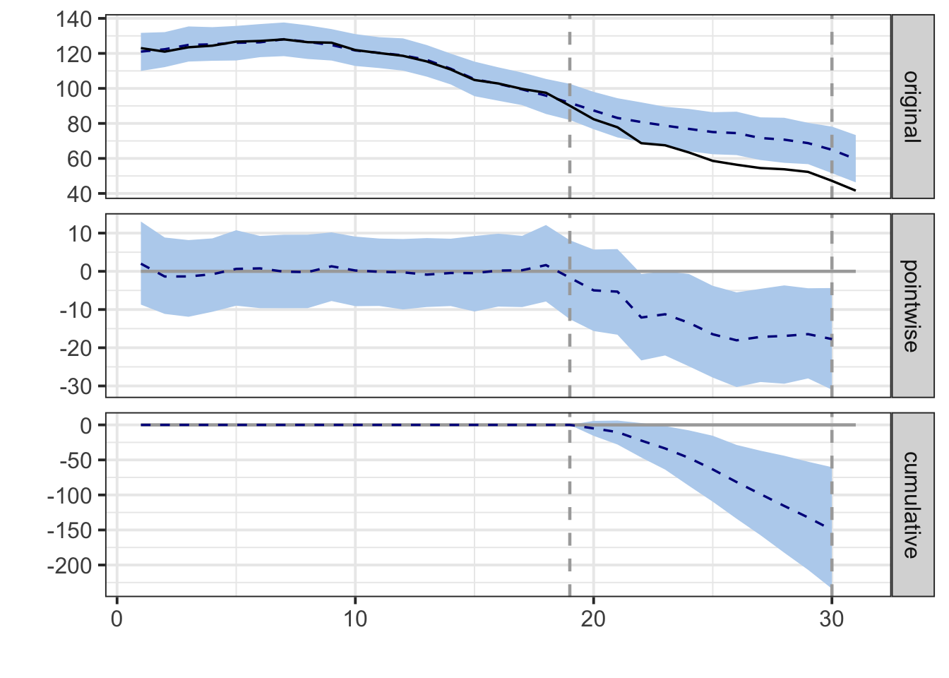
summary(impact)## Posterior inference {CausalImpact}
##
## Average Cumulative
## Actual 62 683
## Prediction (s.d.) 76 (4.2) 832 (46.2)
## 95% CI [68, 83] [743, 916]
##
## Absolute effect (s.d.) -14 (4.2) -150 (46.2)
## 95% CI [-21, -5.5] [-234, -60.3]
##
## Relative effect (s.d.) -18% (5.5%) -18% (5.5%)
## 95% CI [-28%, -7.2%] [-28%, -7.2%]
##
## Posterior tail-area probability p: 0.00203
## Posterior prob. of a causal effect: 99.79737%
##
## For more details, type: summary(impact, "report")还有一种思路,我们选一些和加州最像的州来作为CausalImpact的解释变量,或者加入更多外部解释变量,比如我们加入加州香烟价格
library(CausalImpact)
library(tidyverse)
library(zoo)
library(anytime)
str(aggdata) ## 'data.frame': 62 obs. of 17 variables:
## $ Group.1 : num 0 1 0 1 0 1 0 1 0 1 ...
## $ Group.2 : num 1970 1970 1971 1971 1972 ...
## $ uid : num 604 63 605 64 606 ...
## $ year : num 1970 1970 1971 1971 1972 ...
## $ state : num NA NA NA NA NA NA NA NA NA NA ...
## $ cigsale : num 120 123 124 121 129 ...
## $ lnincome : num NaN NaN NaN NaN 9.68 ...
## $ beer : num NaN NaN NaN NaN NaN NaN NaN NaN NaN NaN ...
## $ age15to24 : num 0.178 0.178 0.179 0.179 0.181 ...
## $ retprice : num 35.9 38.8 37.9 39.7 39.3 ...
## $ time : num 0 0 1 1 2 2 3 3 4 4 ...
## $ california : num 0 1 0 1 0 1 0 1 0 1 ...
## $ cal_trend : num 0 0 0 1 0 2 0 3 0 4 ...
## $ tax_dummy : num 0 0 0 0 0 0 0 0 0 0 ...
## $ tax_trend : num 0 0 0 0 0 0 0 0 0 0 ...
## $ cal_tax_dummy: num 0 0 0 0 0 0 0 0 0 0 ...
## $ cal_tax_trend: num 0 0 0 0 0 0 0 0 0 0 ...#在前面的基础上,继续加入加州本身的香烟价格
cig_c_Cas <- cig_c %>% dplyr::select(cigsale,time,retprice)
cont_cig <- aggdata  %>% filter( `Group.1`== 0) %>% dplyr::select(cigsale,time)
data <- left_join(x = cig_c_Cas,y = cont_cig,by="time")
#这里我将其他地区的香烟销量作为预测加州销量的解释变量
pre.period <- c(0, 19)
post.period <- c(20, 30)

impact <- CausalImpact(data, pre.period ,post.period)
## Warning in FormatInputPrePostPeriod(pre.period, post.period, data): Setting
## pre.period[1] to start of data: 1plot(impact)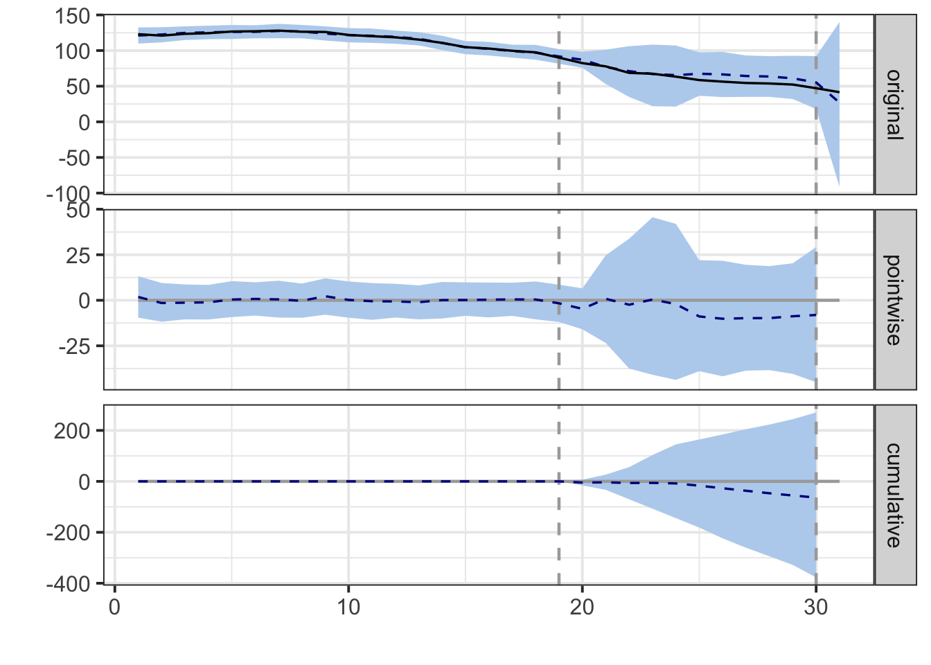
summary(impact)## Posterior inference {CausalImpact}
##
## Average Cumulative
## Actual 62 683
## Prediction (s.d.) 68 (15) 746 (160)
## 95% CI [37, 96] [412, 1060]
##
## Absolute effect (s.d.) -5.8 (15) -63.5 (160)
## 95% CI [-34, 25] [-377, 270]
##
## Relative effect (s.d.) -8.5% (21%) -8.5% (21%)
## 95% CI [-51%, 36%] [-51%, 36%]
##
## Posterior tail-area probability p: 0.34068
## Posterior prob. of a causal effect: 66%
##
## For more details, type: summary(impact, "report")如果加入了香烟价格,可能法案就没有什么效果了,不过这样的分析可能是有问题的,因为估计法令就是直接作用与retprice的。
CausalImpact包估计用来分析股票,可能有点意思,一些重大事件的影响。