聚类分析

什么是聚类？？一个简单的例子

探索性数据分析（EDA）的一种形式,将样本通过特征划分成具有共同特征的有意义的族群。

聚类分析的全部流程图

流程

定义距离和相似性

$距离 = 1 - 相似性$

距离的直观定义

$距离 = \sqrt{{(X_{red} - X_{blue})}^{2} + {(Y_{red} - Y_{blue})}^{2}}$

pacman::p_load(tidyverse,ggthemes,ggfortify,DT)

two_person <- tribble(~x, ~y,
                      0,0,
                      9,12)
ggplot(two_person, aes(x = x, y = y)) + 
  geom_point() +
  lims(x = c(-30,30), y = c(-20, 20)) + theme_clean()+ggtitle("原始数据")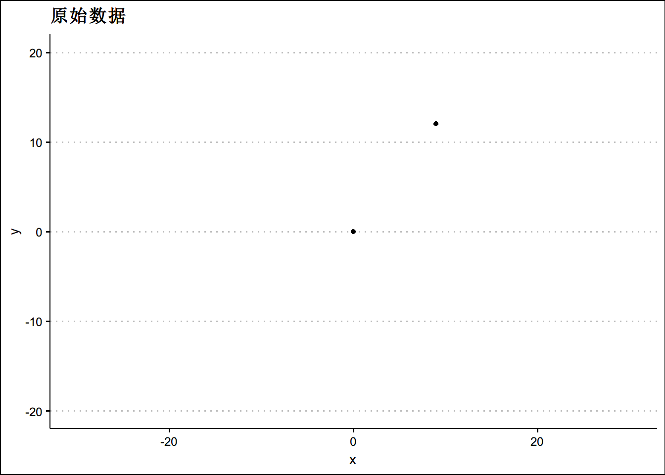

dist(two_person,method = "euclidean")

##    1
## 2 15

多余两个人时

three_p <- tribble(~x, ~y,
                      0,0,
                      9,12,
                   -2,9)
ggplot(three_p, aes(x = x, y = y)) + 
  geom_point() +
  lims(x = c(-30,30), y = c(-20, 20)) + theme_clean()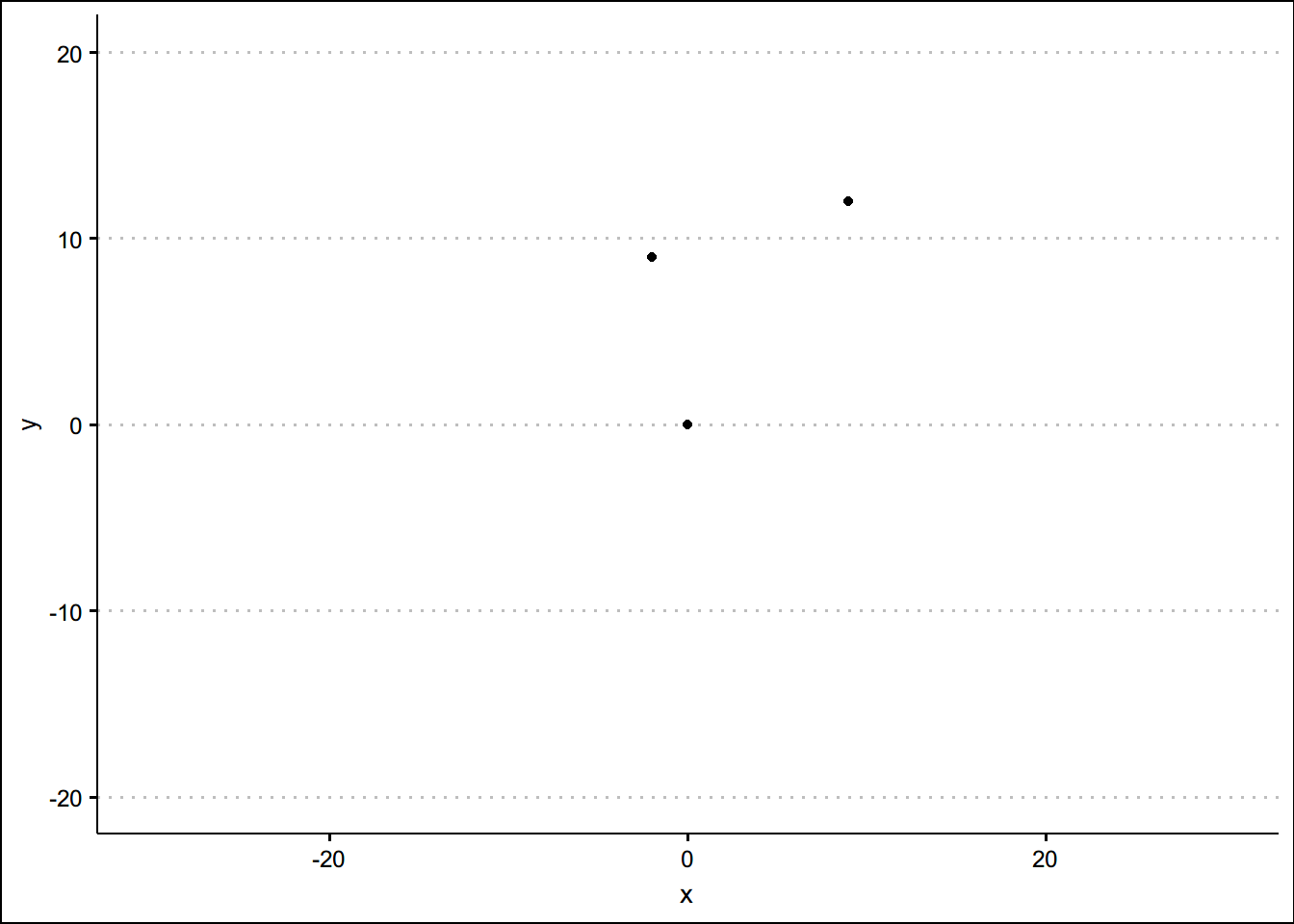

dist(three_p,method = "euclidean")

##           1         2
## 2 15.000000          
## 3  9.219544 11.401754

大家思考一下 1和2,2和3,1和3哪个离得最近（相近性）最高？

数据尺度(scale)的影响

我们在计算样本特征的相似度时，需要注意数据尺度的影响

three_person <- tribble(~weight,~height,
                      8.3,840,
                      8.6,780,
                      10.5,864)
three_person %>% datatable()

	weight	height
1	8.3	840
2	8.6	780
3	10.5	864

{height}_{scaled} = \frac{height - mean(height)}{sd (height)}

dist(three_person)

##          1        2
## 2 60.00075         
## 3 24.10062 84.02149

scale(three_person)

##          weight     height
## [1,] -0.6984984  0.2773501
## [2,] -0.4470390 -1.1094004
## [3,]  1.1455375  0.8320503
## attr(,"scaled:center")
##     weight     height 
##   9.133333 828.000000 
## attr(,"scaled:scale")
##    weight    height 
##  1.193035 43.266615

dist(scale(three_person))

##          1        2
## 2 1.409365         
## 3 1.925659 2.511082

上面一个简单的例子，我们可以看出数据的尺度对我们计算距离有很大影响。

如何计算类别变量(categorical)的距离

我们还是看一个例子

kouwei <- tribble(~la,~suan,~tian,~chou,
                  T,T,F,F,
                  F,T,T,T,
                  T,T,F,T)
kouwei %>% datatable()

	la	suan	tian	chou
1	true	true	false	false
2	false	true	true	true
3	true	true	false	true

如何计算上述口味例子的距离呢？

首先我们定义 $J (A, B) = \frac{A \cap B}{A \cup B}$ 来计算类别型变量的相似度
假设我们希望计算样本1和样本2的距离，根据上面的定义，我们有 $J (1, 2) = \frac{1 \cap 2}{1 \cup 2} = \frac{1}{4}$ 那么1和2的距离为 $1 - J (1, 2) = 1 - \frac{1}{4} = 0.75$ 如果使用软件计算

dist(kouwei,method = 'binary')

##           1         2
## 2 0.7500000          
## 3 0.3333333 0.5000000

如果类别变量多于两个，如何计算距离与相似度？如果你的数据如下，如何处理？

teacher_sat <- tribble(~taidu,~fangfa,~renpin,
                       'high','low','high',
                       'low','high','mid',
                       'mid','mid','mid')
teacher_sat %>% datatable()

	taidu	fangfa	renpin
1	high	low	high
2	low	high	mid
3	mid	mid	mid

面对上述类型的数据，我们需要将多种类型数据处理成虚拟变量，才能进行距离和相似度的计算

library(dummies)
teacher_sat_df <- as.data.frame(teacher_sat) 
teacher_sat_dum <- dummy.data.frame(teacher_sat_df)
teacher_sat_dum

##   taiduhigh taidulow taidumid fangfahigh fangfalow fangfamid renpinhigh
## 1         1        0        0          0         1         0          1
## 2         0        1        0          1         0         0          0
## 3         0        0        1          0         0         1          0
##   renpinmid
## 1         0
## 2         1
## 3         1

dist(teacher_sat_dum,method = 'binary')

##     1   2
## 2 1.0    
## 3 1.0 0.8

teacher_sat

## # A tibble: 3 x 3
##   taidu fangfa renpin
##   <chr> <chr>  <chr> 
## 1 high  low    high  
## 2 low   high   mid   
## 3 mid   mid    mid

如果我们有如下距离矩阵，请思考以下问题：

	1	2	3
2	11.7
3	16.8	18
4	10	20.6	15.8

首先可以肯定的是我们知道样本1和样本4的距离最近
样本2离group 1,4更近？还是样本3离group 1,4更近？
如何判断上述问题的距离？

一种想法： $max (D (2, 1), D (2, 4)) = 20.6$ ， $max (D (3, 1), D (3, 4)) = 16.8$ ，那么3离group1,4比2更近一些。

图解层次聚类

接下来我们扩展一下这个思路，再多放几个队员上场，假设我们现在有6个队员，他们的x坐标和y轴坐标为：

player	x	y
1	-1	1
2	-2	-3
3	8	6
4	7	-8
5	-12	8
6	-15	0

根据以上数据，我们对上面6个球员进行层次聚类Hierarchical clustering

player_6 <- tribble(~x,~y,
                    -1,1,
                    -2,-3,
                    8,6,
                    7,-8,
                    -12,8,
                    -15,0
                    )
# 看一眼球员的位置
ggplot(player_6,aes(x=x,y=y))+geom_point()+theme_clean()+ggtitle("原始数据")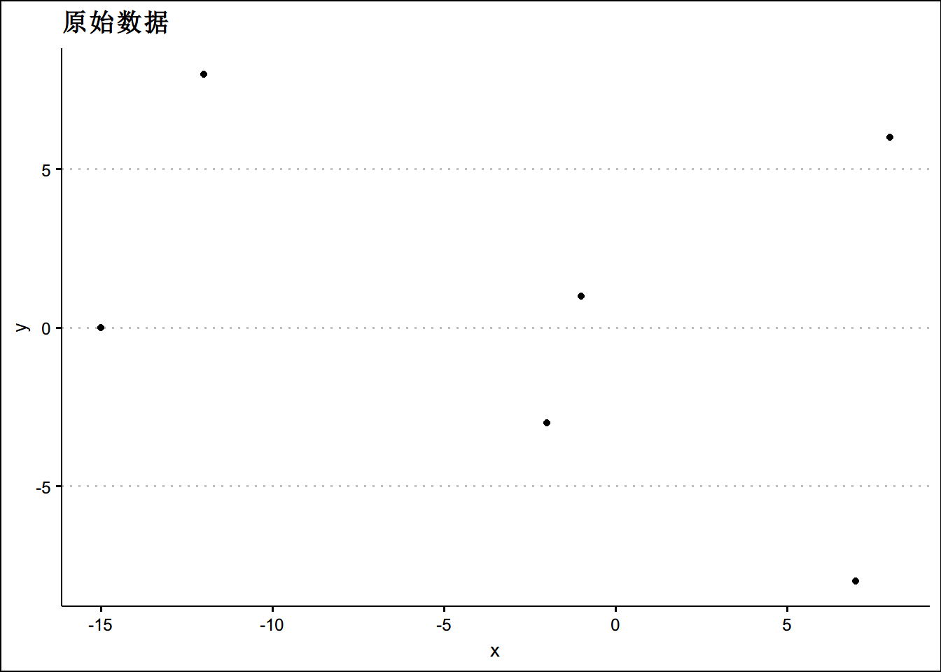

dist_players <- dist(player_6, method = 'euclidean')
hc_players <- hclust(dist_players, method = 'complete')
#如果我们要将数据分成两组,用cuttree剪树枝，这里我手画一个图给大家理解
cluster_assignments <- cutree(hc_players, k = 2)
# 把2组分类的标准装回数据框
play_6_k2 <- player_6 %>%
  mutate(group = cluster_assignments)

ggplot(data = play_6_k2 ,aes(x=x,y=y,color=as.factor(group)))+geom_point(size=3)+theme_clean()+
  ggtitle('分两组情况')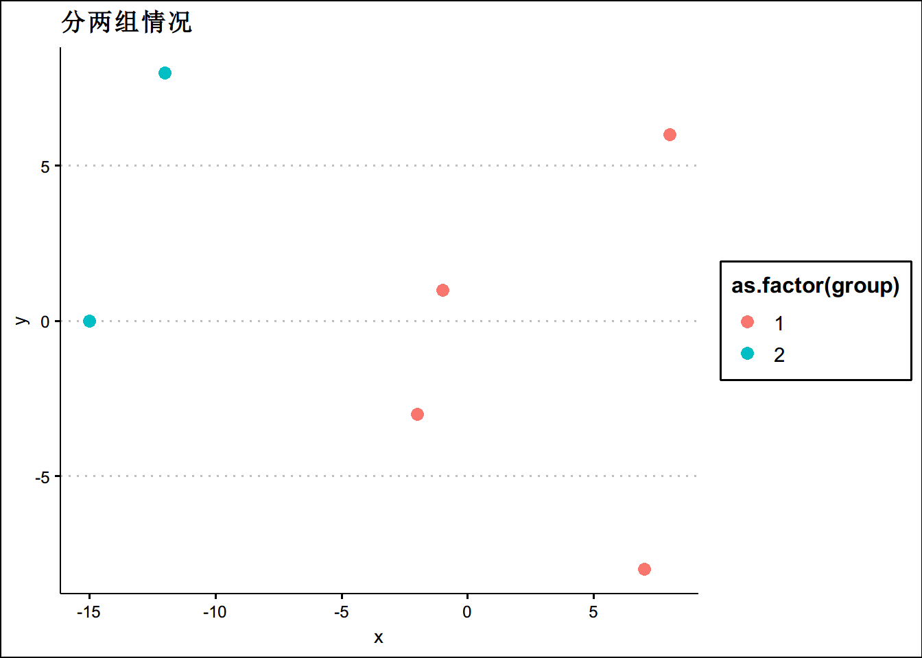

cluster_assignments <- cutree(hc_players, k = 3)
# 把2组分类的标准装回数据框
play_6_k2 <- player_6 %>%
  mutate(group = cluster_assignments)

ggplot(data = play_6_k2 ,aes(x=x,y=y,color=as.factor(group)))+geom_point(size=3)+theme_clean()+
  ggtitle('分三组情况')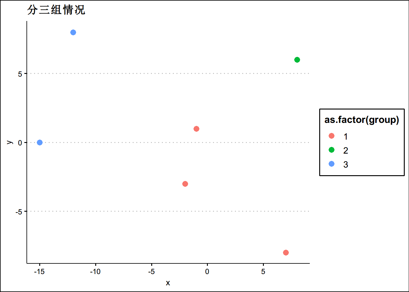

Kmeans的思想：

一个好的聚类算法，应该是能够使得类内的差异尽可能小。设 $W (C_{k})$ 是第 $C_{k}$ 类中差异化的度量，因此我们的问题转化为：

$min {\sum_{k = 1}^{K} W (C_{k})}$

使用平方欧式距离定界定类内差异

$W (C_{k}) = \frac{1}{| C_{k} |} \sum_{i, i^{'} \in C_{k}} {\sum_{j = 1}^{p} (x_{i j} - x_{i^{'} j})}^{2}$ $min {\sum_{k = 1}^{K} \frac{1}{| C_{k} |} {\sum_{i, i^{'} \in C_{k}} \sum_{j = 1}^{p} (x_{i j} - x_{i^{'} j})}^{2}}$

具体算法：

1 随机为每个观测值分配一个1到K的数字

2 遍历所有数据，将每个数据划分到最近的中心点中

3 计算每个聚类的平均值，并作为新的中心点

4 重复2-3，直到这k个中线点不再变化（收敛了），或执行了足够多的迭代

上图展示了K=3的Kmeans聚类算法过程，先给每个观测值随机分配1-3的数字，然后算出这些1-3类的中心，第一行第三个图展示了这个中心；左下第一张图，每个观测值被分配到了与之最接近的类中；第二行第二列图，重新计算不同类的中心；第二行第三列反复迭代后的结果。我们先虚拟一个项目

set.seed(123)
x <- matrix(rnorm(500*2),ncol=2)
x[1:250,1] <- x[1:250,1]+10 #分别加10和减去10
x[1:250,2] <- x[1:250,2]-10
x <- as.tibble(x)
ggplot(data = x ,aes(x=V1,y=V2))+geom_point()+theme_clean()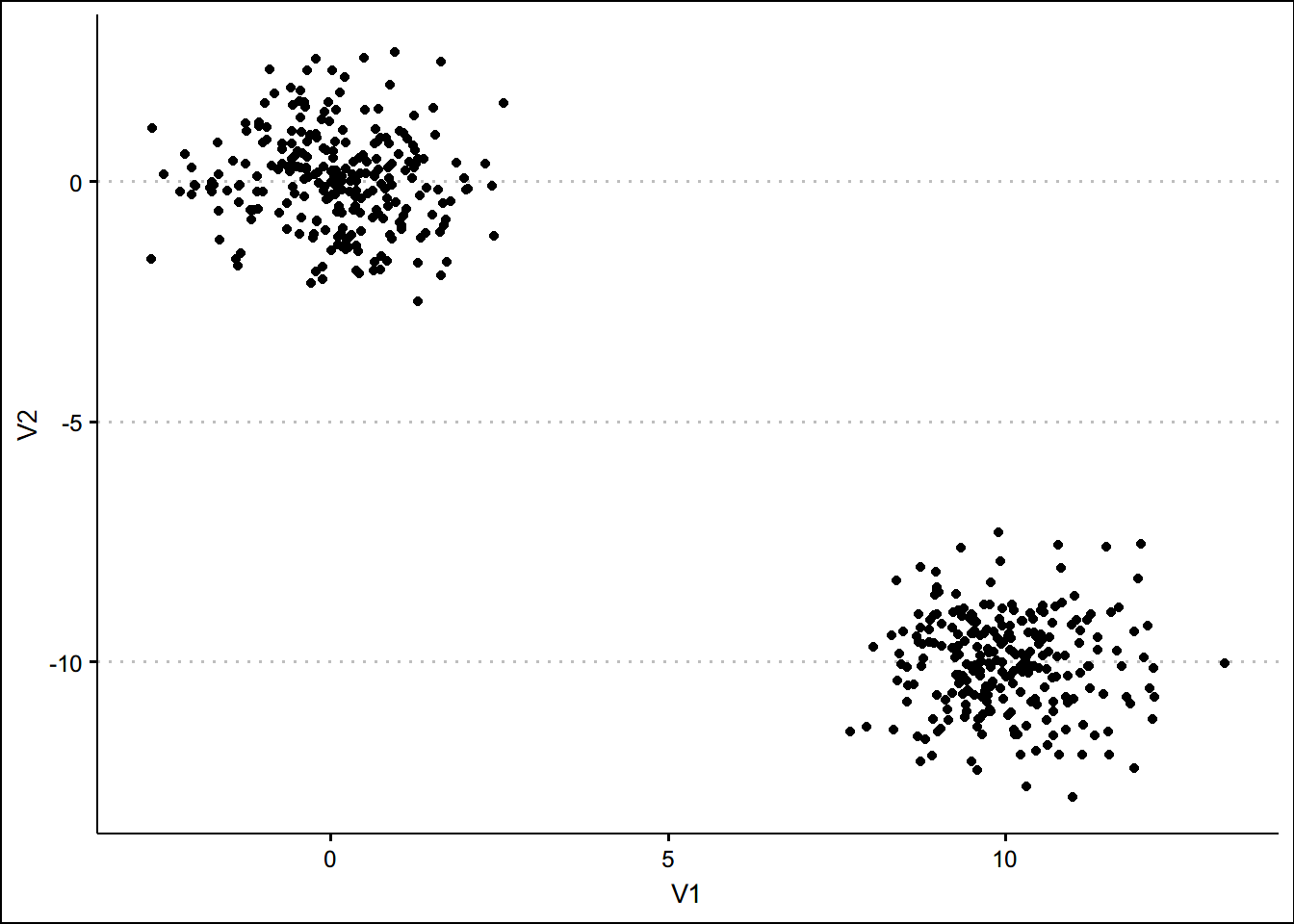

#看一眼数据
km_out <- kmeans(x,centers = 2)
clust_km2 <-km_out$cluster
x_km2 <- mutate(x,cluster = clust_km2)
#再画一下数据
ggplot(data=x_km2,aes(x=V1,y=V2,color=as.factor(clust_km2)))+geom_point()+theme_clean()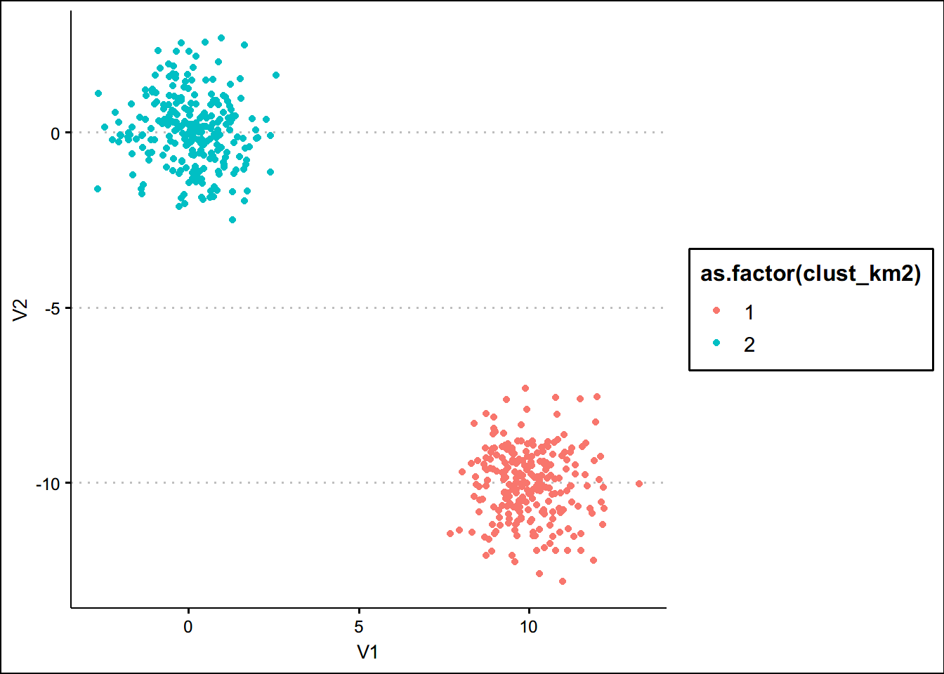

如何选择k，如果我们事前不知道k如何处理？

先看个动图

library(haven)
library(factoextra)
aqi <- read_dta("data/data_0224.dta")
aqi <- aqi %>%
  select(city,aqi ,pm25,pm10,no2,o3,co,so2) %>%
  drop_na() 


aqi_sum <- aqi %>% 
  group_by(city) %>%
  summarise(pm25_m =mean(pm25),so2_m = mean(so2),pm10_m=mean(pm10),no2_m=mean(no2),co_m=mean(co))

rownames(aqi_sum) <- aqi_sum$city
aqi_c <- select(aqi_sum, - city)
km_out <- kmeans(aqi_c,centers = 2)


fviz_cluster(km_out,data=aqi_c) +theme_clean() + ggtitle("k=2的聚类结果")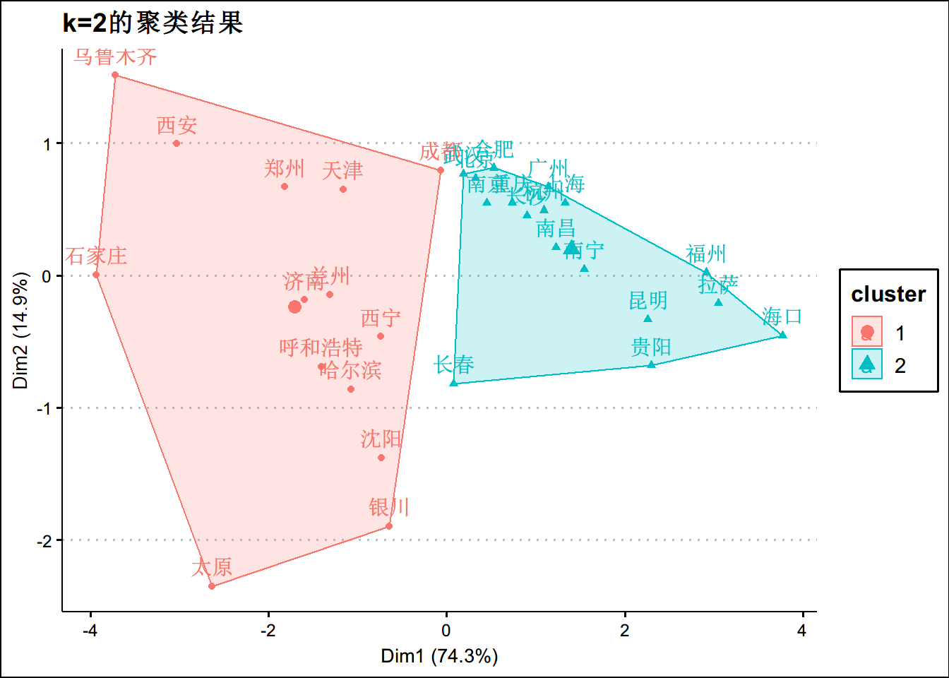

km_out3 <- kmeans(aqi_c,centers = 3)
fviz_cluster(km_out3,data=aqi_c) +theme_clean() + ggtitle("k=3的聚类结果")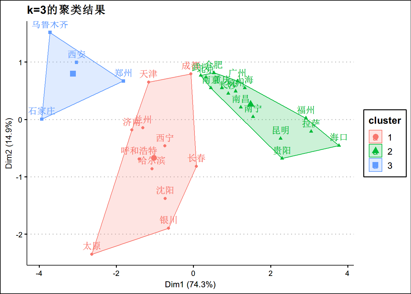

km_out4 <- kmeans(aqi_c,centers = 4)
fviz_cluster(km_out4,data=aqi_c) +theme_clean() + ggtitle("k=4的聚类结果")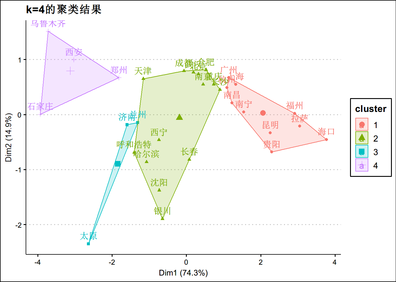

如何寻找最优的k？

Elbow Method

kmean聚类背后的基本思想是定义集群，以使总集群内变化（称为总集群内变化或总集群内平方和）最小化： $minimize (\sum_{k = 1}^{k} W (C_{k}))$ $C_{k}$ 是第 $k^{t h}$ 个集群 $W (C_{k})$ 是集群内的变异。

Elbow Method：

针对k的不同值计算kmean。例如，kmean中选取1到10个集群参数
对于每个k，计算群集内的总平方和（wss）
根据聚类数k绘制wss曲线。
曲线中拐点的位置通常被视为适当簇数的指标。 *** 可以通过以下方法实现

set.seed(123)
wss <- function(k) {
  kmeans(aqi_c, k, nstart = 10 )$tot.withinss
}
k_val <- 1:10
wss_values <- map_dbl(k_val, wss)

plot(k_val, wss_values,
       type="b", pch = 19, frame = FALSE, 
       xlab="Number of clusters K",
       ylab="Total within-clusters sum of squares")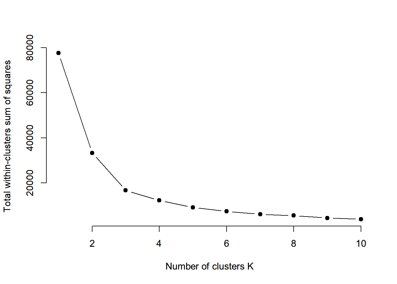

#或者直接用便好的函数

fviz_nbclust(aqi_c, kmeans, method = "wss")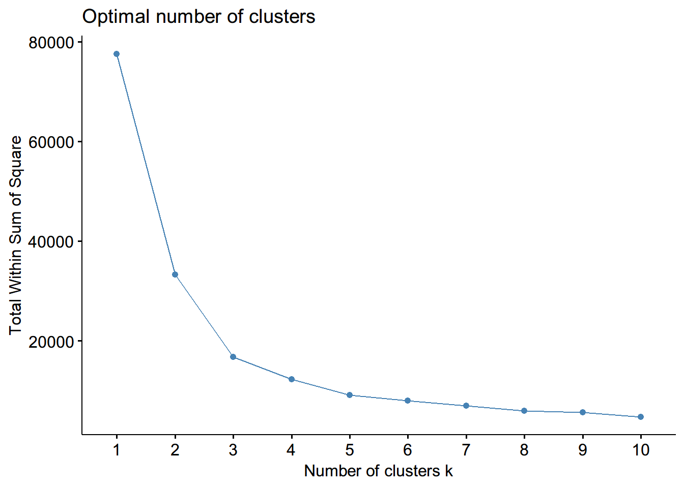

#可能选三是合适的

张剑

2020/03/21