时间序列最简单的预测方法
均值法
\[\hat{y}_{T+h | T}=\left(y_{1}+\cdots+y_{T}\right) / T\]
一个例子
library(tidyverse)## -- Attaching packages ---------------------------------------------------- tidyverse 1.3.0 --## √ ggplot2 3.3.0 √ purrr 0.3.3
## √ tibble 2.1.3 √ dplyr 0.8.5
## √ tidyr 1.0.2 √ stringr 1.4.0
## √ readr 1.3.1 √ forcats 0.5.0## -- Conflicts ------------------------------------------------------- tidyverse_conflicts() --
## x dplyr::filter() masks stats::filter()
## x dplyr::lag() masks stats::lag()library(forecast)## Registered S3 method overwritten by 'quantmod':
## method from
## as.zoo.data.frame zoolibrary(fpp2)## 载入需要的程辑包:fma## 载入需要的程辑包:expsmoothlibrary(ggfortify)## Registered S3 methods overwritten by 'ggfortify':
## method from
## autoplot.Arima forecast
## autoplot.acf forecast
## autoplot.ar forecast
## autoplot.bats forecast
## autoplot.decomposed.ts forecast
## autoplot.ets forecast
## autoplot.forecast forecast
## autoplot.stl forecast
## autoplot.ts forecast
## fitted.ar forecast
## fortify.ts forecast
## residuals.ar forecastlibrary(ggthemes)
library(timetk)
library(DT)
# 设定数据
beer2 <- window(ausbeer,start=1992,end=c(2007,4))
# 均值预测
k<-meanf(beer2,h=11)
k$mean## Qtr1 Qtr2 Qtr3 Qtr4
## 2008 435.375 435.375 435.375 435.375
## 2009 435.375 435.375 435.375 435.375
## 2010 435.375 435.375 435.375beer2_f <- ts.union(beer2,k$mean)
colnames(beer2_f) <- c("原始值",'均值预测')
autoplot(beer2_f,size=1.4,alpha=0.7)+theme_clean()+ggtitle("啤酒销量均值预测")+
xlab("年份")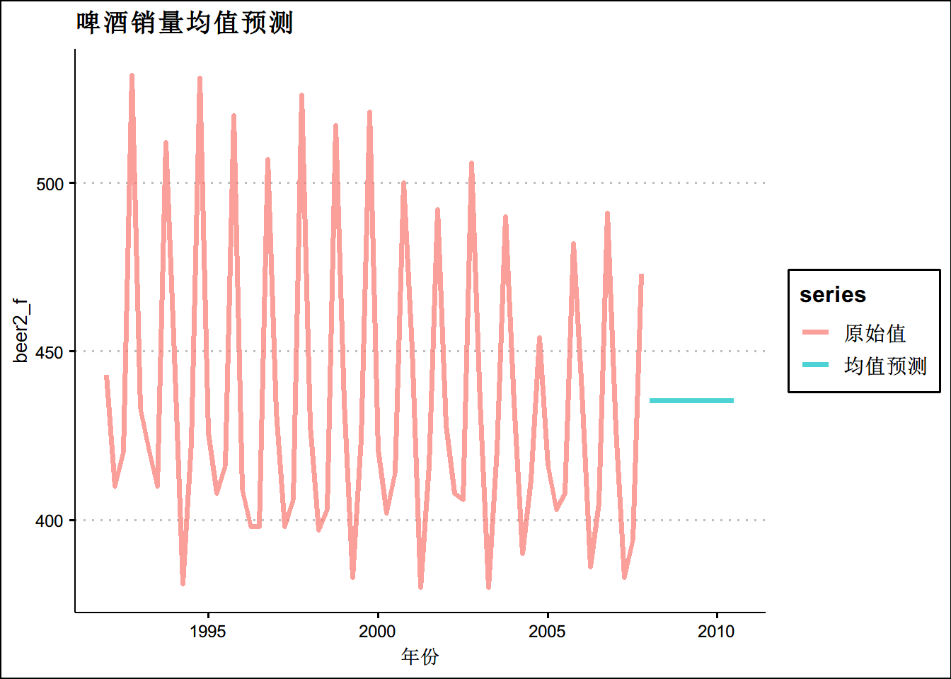
#naive预测
n <- naive(beer2,h=11)
n$mean
## Qtr1 Qtr2 Qtr3 Qtr4
## 2008 473 473 473 473
## 2009 473 473 473 473
## 2010 473 473 473beer2_f <- ts.union(beer2,k$mean,n$mean)
colnames(beer2_f) <- c("原始值",'均值预测','naive预测')
autoplot(beer2_f,size=1.4,alpha=0.7)+theme_clean()+ggtitle("啤酒销量均值预测")+
xlab("年份")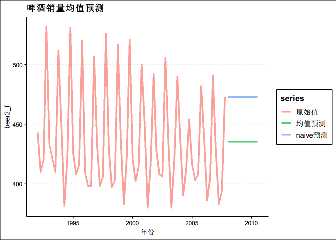
#snaive预测
s_n <- snaive(beer2,h=11)
s_n$mean
## Qtr1 Qtr2 Qtr3 Qtr4
## 2008 427 383 394 473
## 2009 427 383 394 473
## 2010 427 383 394beer2_f <- ts.union(beer2,k$mean,n$mean,s_n$mean)
colnames(beer2_f) <- c("原始值",'均值预测','naive预测','snaive预测')
autoplot(beer2_f,size=1.4,alpha=0.7)+theme_clean()+ggtitle("啤酒销量均值预测")+
xlab("年份")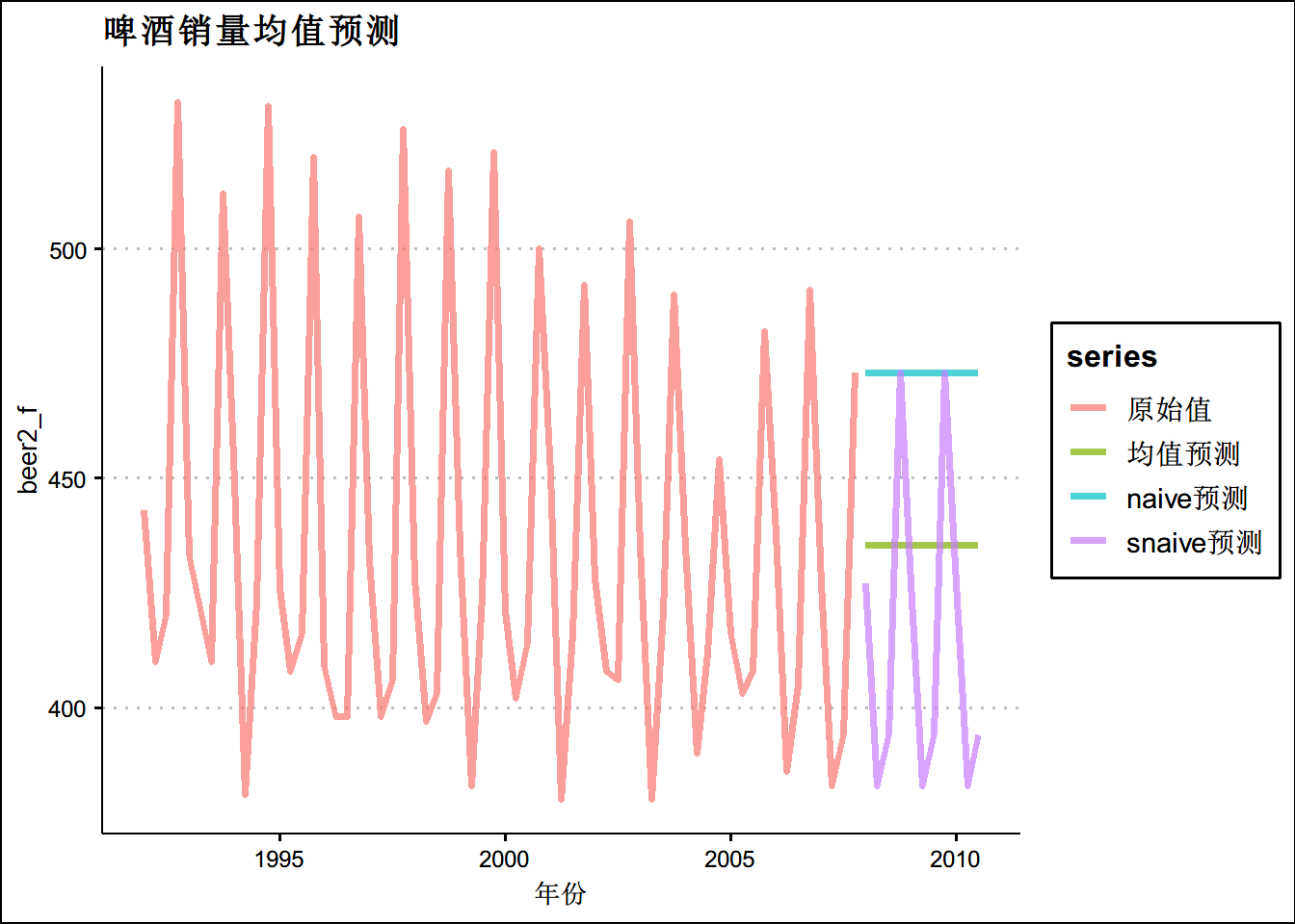
#漂移法
d<- rwf(beer2,h=11,drift = T)
d$mean
## Qtr1 Qtr2 Qtr3 Qtr4
## 2008 473.4762 473.9524 474.4286 474.9048
## 2009 475.3810 475.8571 476.3333 476.8095
## 2010 477.2857 477.7619 478.2381beer2_f <- ts.union(beer2,k$mean,n$mean,s_n$mean,d$mean)
colnames(beer2_f) <- c("原始值",'均值预测','naive预测','snaive预测','漂移法')
autoplot(beer2_f,size=1.4,alpha=0.7)+theme_clean()+ggtitle("啤酒销量均值预测")+
xlab("年份")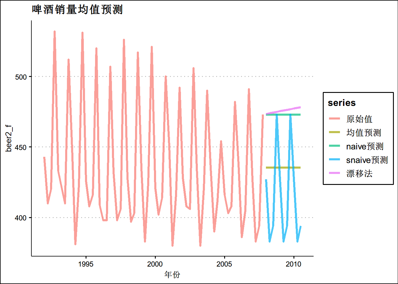
预测精度的例子
beer2 <- window(ausbeer,start=1992,end=c(2007,4))
beerfit1 <- meanf(beer2,h=10)
beerfit2 <- rwf(beer2,h=10)
beerfit3 <- snaive(beer2,h=10)
beer3 <- window(ausbeer, start=2008)
accuracy(beerfit1, beer3)
## ME RMSE MAE MPE MAPE MASE ACF1
## Training set 0.000 43.62858 35.23438 -0.9365102 7.886776 2.463942 -0.10915105
## Test set -13.775 38.44724 34.82500 -3.9698659 8.283390 2.435315 -0.06905715
## Theil's U
## Training set NA
## Test set 0.801254accuracy(beerfit2, beer3)## ME RMSE MAE MPE MAPE MASE
## Training set 0.4761905 65.31511 54.73016 -0.9162496 12.16415 3.827284
## Test set -51.4000000 62.69290 57.40000 -12.9549160 14.18442 4.013986
## ACF1 Theil's U
## Training set -0.24098292 NA
## Test set -0.06905715 1.254009accuracy(beerfit3, beer3)## ME RMSE MAE MPE MAPE MASE ACF1
## Training set -2.133333 16.78193 14.3 -0.5537713 3.313685 1.0000000 -0.2876333
## Test set 5.200000 14.31084 13.4 1.1475536 3.168503 0.9370629 0.1318407
## Theil's U
## Training set NA
## Test set 0.298728#这里我们直接使用autoplayer包
googfc1 <- meanf(goog200, h=40)
googfc2 <- rwf(goog200, h=40)
googfc3 <- rwf(goog200, drift=TRUE, h=40)
autoplot(subset(goog, end = 240)) +
autolayer(googfc1, PI=FALSE, series="均值") +
autolayer(googfc2, PI=F, series="Naïve") +
autolayer(googfc3, PI=FALSE, series="漂移") +
xlab("天") + ylab("收盘价(美元)") +
ggtitle("谷歌公司每日股价(截止至2013年12月6日)") +
guides(colour=guide_legend(title="预测"))+
theme(text = element_text(family = "STHeiti"))+
theme(plot.title = element_text(hjust = 0.5)) +
theme_clean()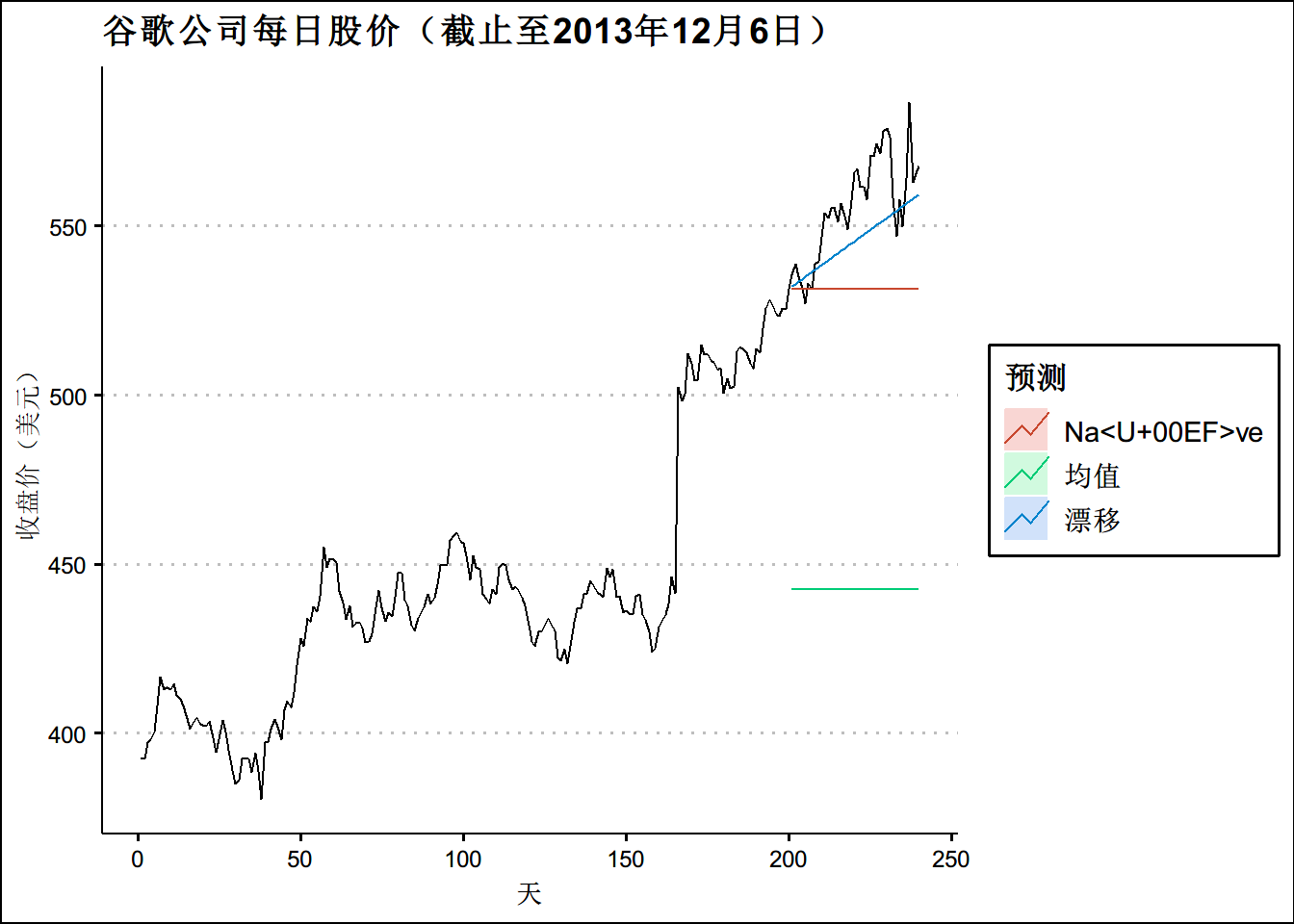
#计算预测精度
googtest <- window(goog, start=201, end=240)
accuracy(googfc1, googtest)
## ME RMSE MAE MPE MAPE MASE
## Training set -4.296286e-15 36.91961 26.86941 -0.6596884 5.95376 7.182995
## Test set 1.132697e+02 114.21375 113.26971 20.3222979 20.32230 30.280376
## ACF1 Theil's U
## Training set 0.9668981 NA
## Test set 0.8104340 13.92142accuracy(googfc2, googtest)## ME RMSE MAE MPE MAPE MASE
## Training set 0.6967249 6.208148 3.740697 0.1426616 0.8437137 1.000000
## Test set 24.3677328 28.434837 24.593517 4.3171356 4.3599811 6.574582
## ACF1 Theil's U
## Training set -0.06038617 NA
## Test set 0.81043397 3.451903accuracy(googfc3, googtest)## ME RMSE MAE MPE MAPE MASE
## Training set -5.998536e-15 6.168928 3.824406 -0.01570676 0.8630093 1.022378
## Test set 1.008487e+01 14.077291 11.667241 1.77566103 2.0700918 3.119002
## ACF1 Theil's U
## Training set -0.06038617 NA
## Test set 0.64732736 1.709275移动平均,简单移动平均的阶数常常是奇数阶,在阶数为m=2k+1的移动平均中,中心值两侧各有k个观测值可以被平均
先看一个白噪声的例子
set.seed(3)
wn <- ts(rnorm(36))
autoplot(wn,size =1.1,alpha = 0.7)+theme_clean()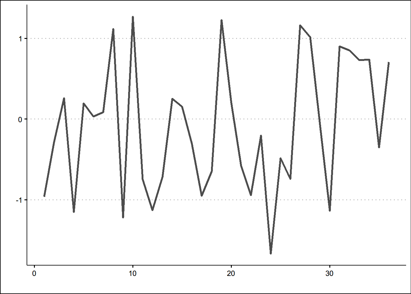
autoplot(mstl(wn))+theme_clean()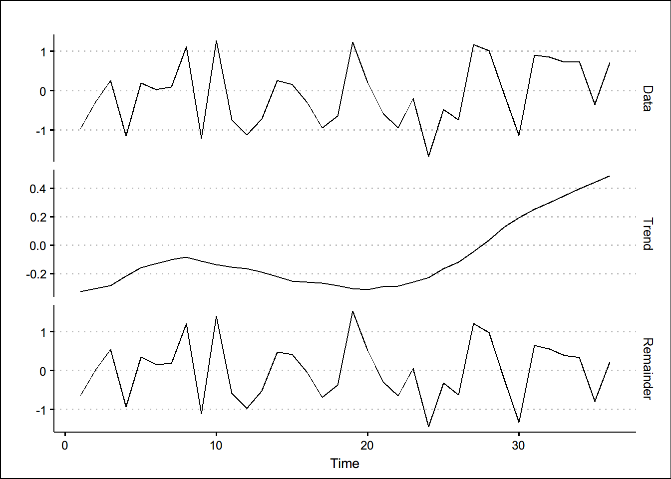
data(elecsales)
ele <- timetk::tk_tbl(elecsales)

ele <- ele %>%
  mutate(mm = ma(elecsales,order = 5))
ele %>% datatable(colnames = c("年份","原始数据","MA5"))
#ma5第一个数是2381.53,具体计算方式如下:
paste("这个数是这样得到的:",mean(pull(ele[1:5,'value'])),"下面会显示一个TRUE")## [1] "这个数是这样得到的: 2381.53 下面会显示一个TRUE"ele[3,3]==mean(pull(ele[1:5,'value']))## mm
## [1,] TRUE#ma5图
autoplot(elecsales,size=1.5,alpha=0.6 ,series="原始数据") +
autolayer(ma(elecsales,5), series="5-MA",size=1.5,alpha=0.6) +
xlab("年份") + ylab("亿瓦时") +
ggtitle("年度住宅售电量") +
scale_colour_manual(values=c("Data"="grey50","5-MA"="red"),
breaks=c("Data","5-MA"))+
theme(text = element_text(family = "STHeiti"))+
theme(plot.title = element_text(hjust = 0.5))+theme_clean()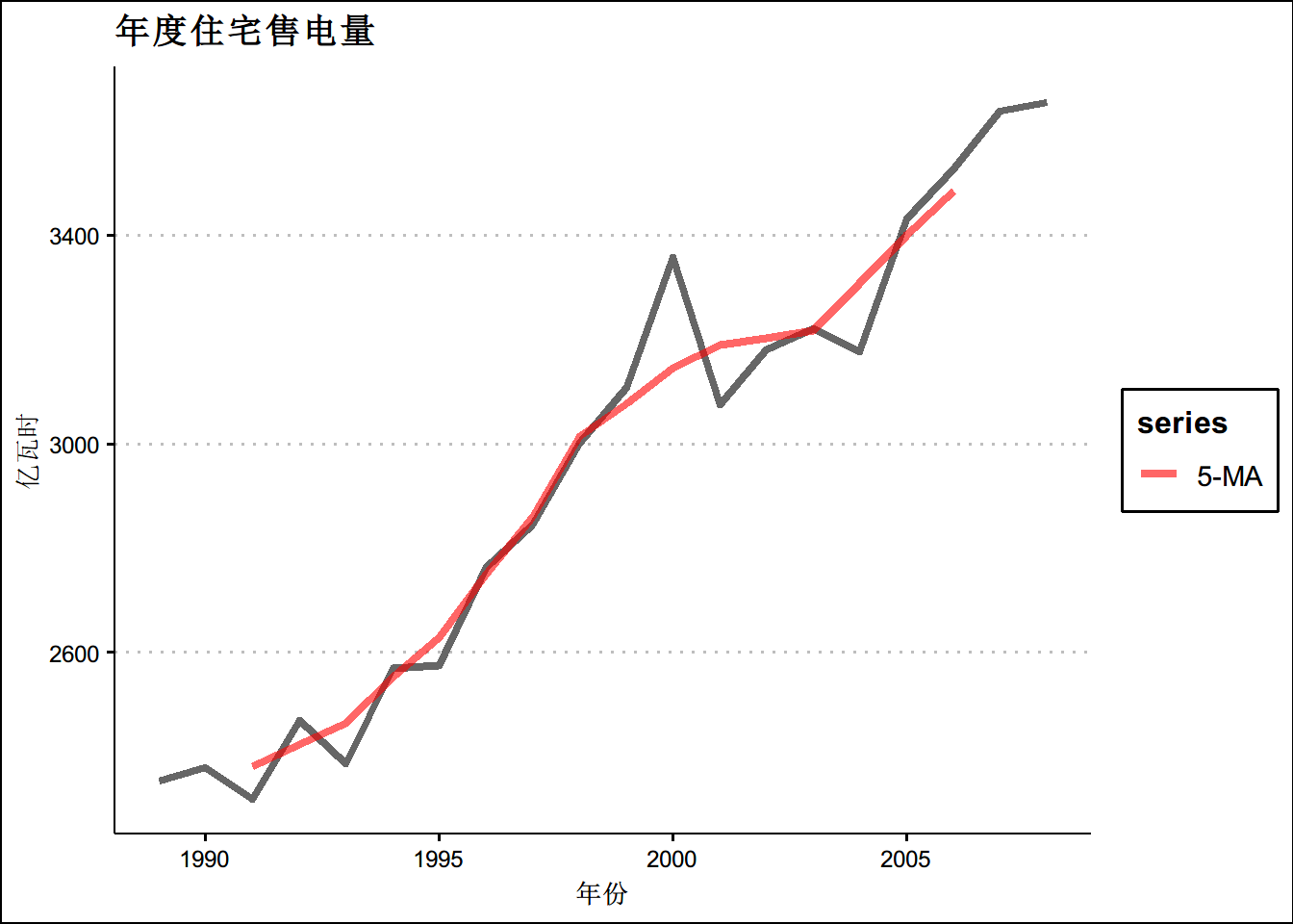
#ma3图
autoplot(elecsales,size=1.5,alpha=0.6 ,series="原始数据") +
  autolayer(ma(elecsales,3), series="3-MA",size=1.5,alpha=0.6) +
  xlab("年份") + ylab("亿瓦时") +
  ggtitle("年度住宅售电量") +
  scale_colour_manual(values=c("Data"="grey50","3-MA"="red"),
                     breaks=c("Data","3-MA"))+
  theme(text = element_text(family = "STHeiti"))+
  theme(plot.title = element_text(hjust = 0.5))+theme_clean()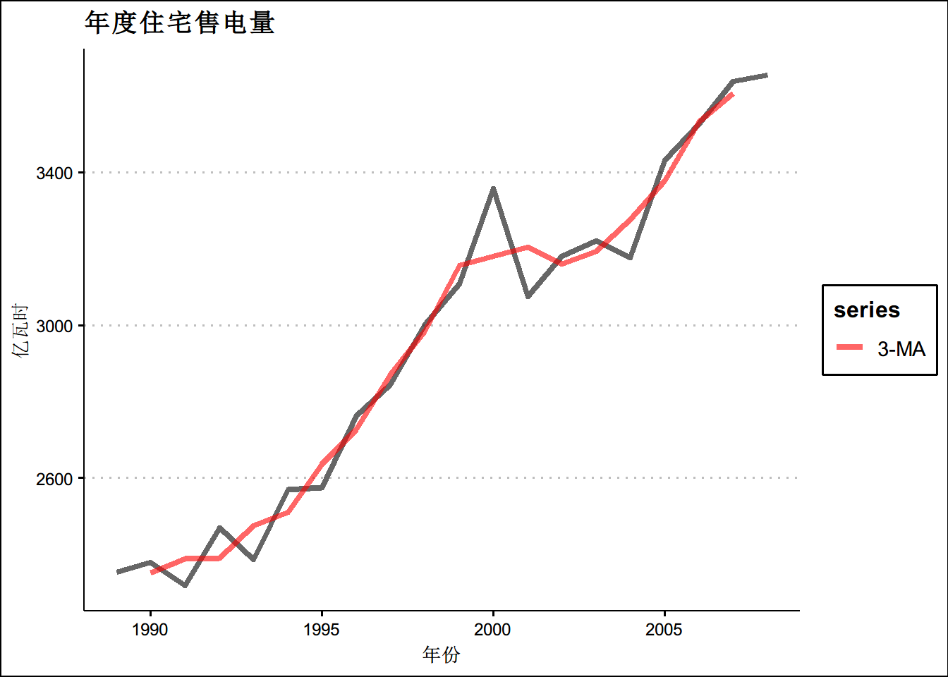
#ma3图
autoplot(elecsales,size=1.5,alpha=0.6 ,series="原始数据") +
autolayer(ma(elecsales,7), series="7-MA",size=1.5,alpha=0.6) +
xlab("年份") + ylab("亿瓦时") +
ggtitle("年度住宅售电量") +
scale_colour_manual(values=c("Data"="grey50","7-MA"="red"),
breaks=c("Data","7-MA"))+
theme(text = element_text(family = "STHeiti"))+
theme(plot.title = element_text(hjust = 0.5))+theme_clean()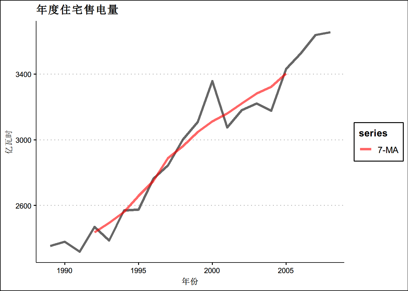 ## 移动平均的移动平均
beer2 <- window(ausbeer,start=1992)
beer2_df <- timetk::tk_tbl(beer2)

beer2_df <- beer2_df %>%
  mutate(mm = ma(beer2,order = 4,centre = F)) %>%
  mutate(mmm = ma(beer2,order = 4,centre = T))
beer2_df %>% datatable(colnames = c("年份","原始数据","MA4","2*4MA"))
# 450 = (451.25+448.75)/2使用线性模型对时间序列进行预测
\[y_{t}=\beta_{0}+\beta_{1} t+\beta_{2} d_{2, t}+\beta_{3} d_{3, t}+\beta_{4} d_{4, t}+\varepsilon_{t}\]
beer2 <- window(ausbeer, start=1992)
fit.beer <- tslm(beer2 ~ trend + season)
summary(fit.beer)
##
## Call:
## tslm(formula = beer2 ~ trend + season)
##
## Residuals:
## Min 1Q Median 3Q Max
## -42.903 -7.599 -0.459 7.991 21.789
##
## Coefficients:
## Estimate Std. Error t value Pr(>|t|)
## (Intercept) 441.80044 3.73353 118.333 < 2e-16 ***
## trend -0.34027 0.06657 -5.111 2.73e-06 ***
## season2 -34.65973 3.96832 -8.734 9.10e-13 ***
## season3 -17.82164 4.02249 -4.430 3.45e-05 ***
## season4 72.79641 4.02305 18.095 < 2e-16 ***
## ---
## Signif. codes: 0 '***' 0.001 '**' 0.01 '*' 0.05 '.' 0.1 ' ' 1
##
## Residual standard error: 12.23 on 69 degrees of freedom
## Multiple R-squared: 0.9243, Adjusted R-squared: 0.9199
## F-statistic: 210.7 on 4 and 69 DF, p-value: < 2.2e-16#拟合完了
#画图
beer2_f <- ts.union(beer2,fitted(fit.beer))
colnames(beer2_f) <- c("原始值",'拟合值')
autoplot(beer2_f, series="真实值",size=1,alpha=0.8) +
xlab("年份") + ylab("万升") +
ggtitle("啤酒的季度产出")+
theme(text = element_text(family = "STHeiti"))+
theme(plot.title = element_text(hjust = 0.5)) +
theme_clean()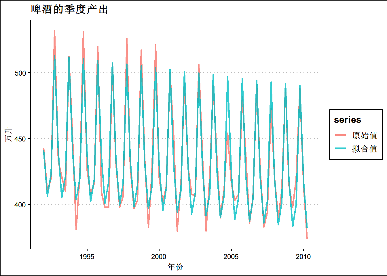
cbind(Data=beer2, Fitted=fitted(fit.beer)) %>%
  as.data.frame() %>%
  ggplot(aes(x=Data, y=Fitted, colour=as.factor(cycle(beer2)))) +
    geom_point() +
    ylab("拟合值") + xlab("真实值") +
    ggtitle("啤酒的季度产出") +
    scale_colour_brewer(palette="Dark2", name="季度") +
    geom_abline(intercept=0, slope=1)+
    theme(text = element_text(family = "STHeiti"))+
    theme(plot.title = element_text(hjust = 0.5))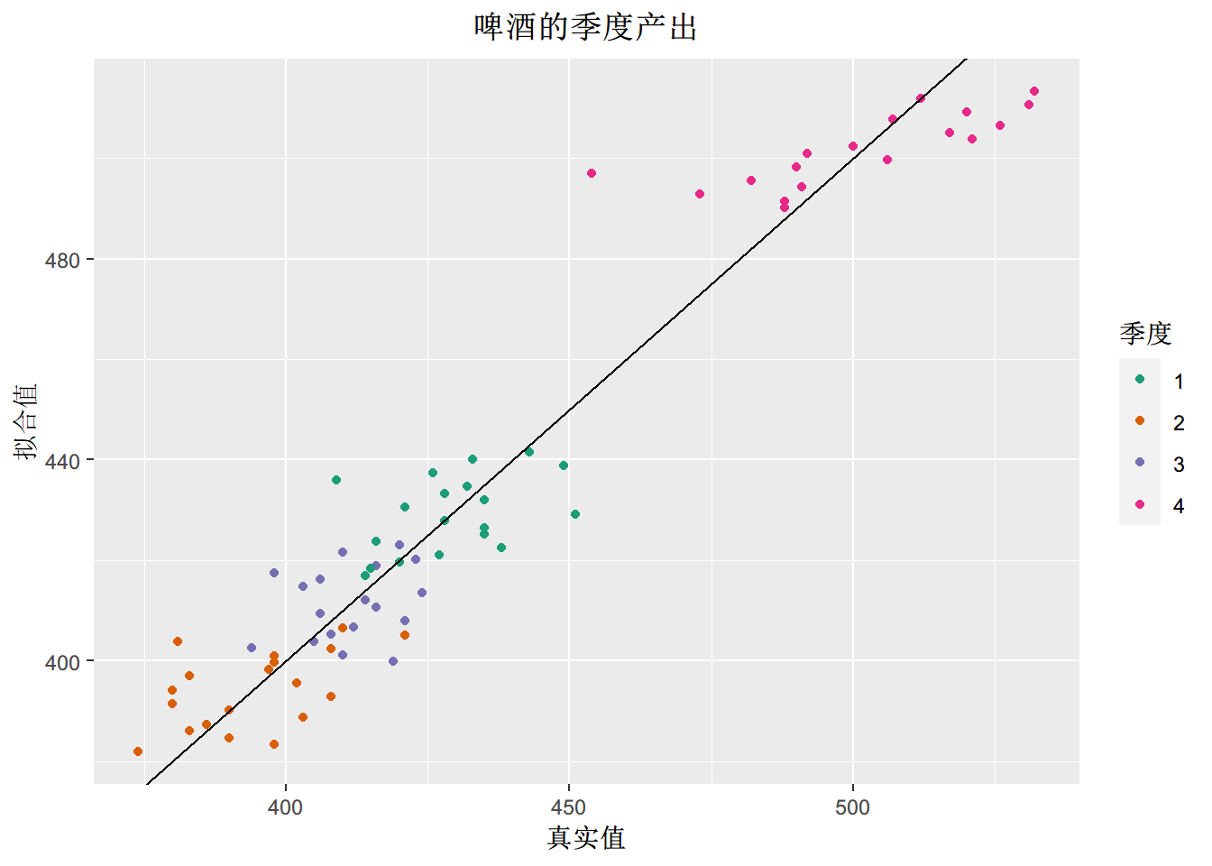
使用拟合好的模型进行预测
beer2 <- window(ausbeer, start=1992)
ggAcf(beer2)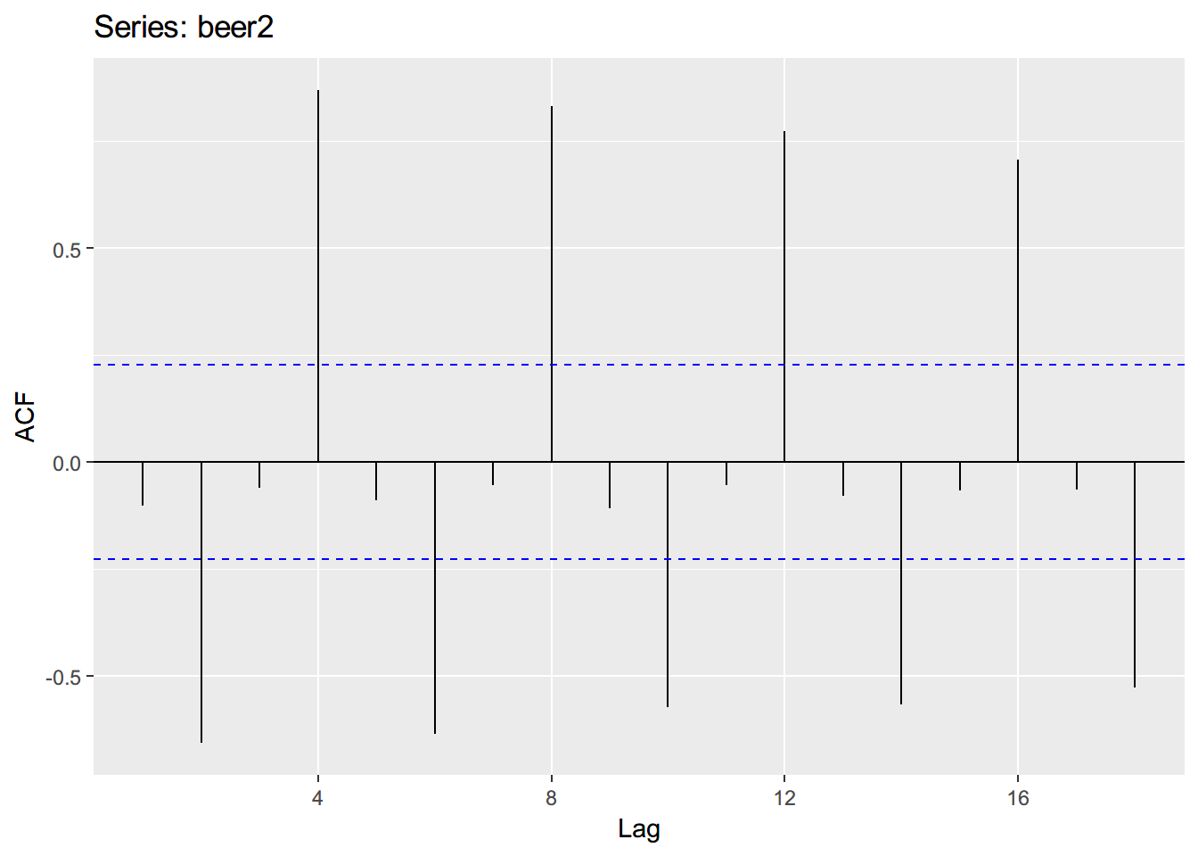
fit.beer <- tslm(beer2 ~ trend + season)
fcast <- forecast(fit.beer)
summary(fcast)
##
## Forecast method: Linear regression model
##
## Model Information:
##
## Call:
## tslm(formula = beer2 ~ trend + season)
##
## Coefficients:
## (Intercept) trend season2 season3 season4
## 441.8004 -0.3403 -34.6597 -17.8216 72.7964
##
##
## Error measures:
## ME RMSE MAE MPE MAPE MASE
## Training set -1.536051e-15 11.80909 9.029722 -0.06895219 2.08055 0.665348
## ACF1
## Training set -0.2499017
##
## Forecasts:
## Point Forecast Lo 80 Hi 80 Lo 95 Hi 95
## 2010 Q3 398.4587 381.8746 415.0428 372.8900 424.0274
## 2010 Q4 488.7365 472.1524 505.3206 463.1678 514.3052
## 2011 Q1 415.5998 399.0029 432.1968 390.0113 441.1883
## 2011 Q2 380.5998 364.0029 397.1968 355.0113 406.1883
## 2011 Q3 397.0976 380.4421 413.7532 371.4188 422.7765
## 2011 Q4 487.3754 470.7199 504.0310 461.6966 513.0543
## 2012 Q1 414.2387 397.5669 430.9106 388.5347 439.9428
## 2012 Q2 379.2387 362.5669 395.9106 353.5347 404.9428
## 2012 Q3 395.7366 379.0028 412.4704 369.9371 421.5360
## 2012 Q4 486.0143 469.2806 502.7481 460.2149 511.8138autoplot(fcast) +
ggtitle("利用线性回归模型预测啤酒产出")+
theme(text = element_text(family = "STHeiti"))+
theme(plot.title = element_text(hjust = 0.5)) + theme_clean()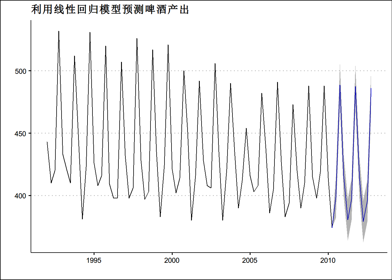
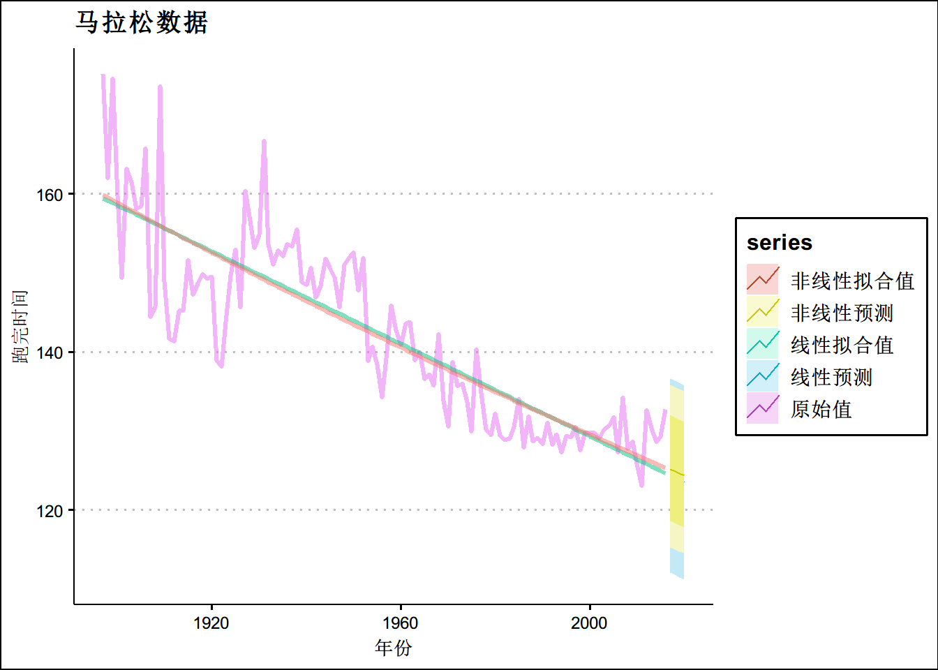
autoplot(marathon,size=1.1,alpha = 0.5,ts.colour = "dodgerblue3")+theme_clean()+
  ggtitle("马拉松数据")+
  xlab("年份")+
  ylab("跑完用时")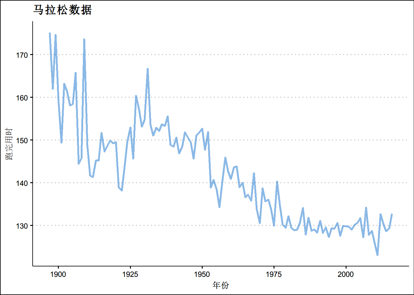
#异方差现象library(forecast)
h <- 4 # 预测四期
fit.lin <- tslm(marathon ~ trend )
fcasts.lin <- forecast(fit.lin, h = h)
fit.exp <- tslm(marathon ~ trend , lambda = 0)
fcasts.exp <- forecast(fit.exp, h = h)
marathon_f <- ts.union(marathon,fitted(fit.lin),fitted(fit.exp))
colnames(marathon_f) <- c("原始值",'线性拟合值','非线性拟合值')
autoplot(marathon_f,size=1.1,alpha=0.5) +
ggtitle("利用线性回归模型预测啤酒产出")+
theme(text = element_text(family = "STHeiti"))+
theme(plot.title = element_text(hjust = 0.5)) + theme_clean()+
autolayer(fcasts.lin, series = '线性预测')+
autolayer(fcasts.exp,series = '非线性预测') +xlab('年份')+ylab('跑完时间')+
ggtitle("马拉松数据")