一些直观的时间序列
library(tidyverse)
library(forecast)
library(fpp2)
library(ggfortify)
library(ggthemes)
autoplot(ausbeer,ts.colour = "blue",main = "啤酒销量",xlab = "时间")+theme_clean()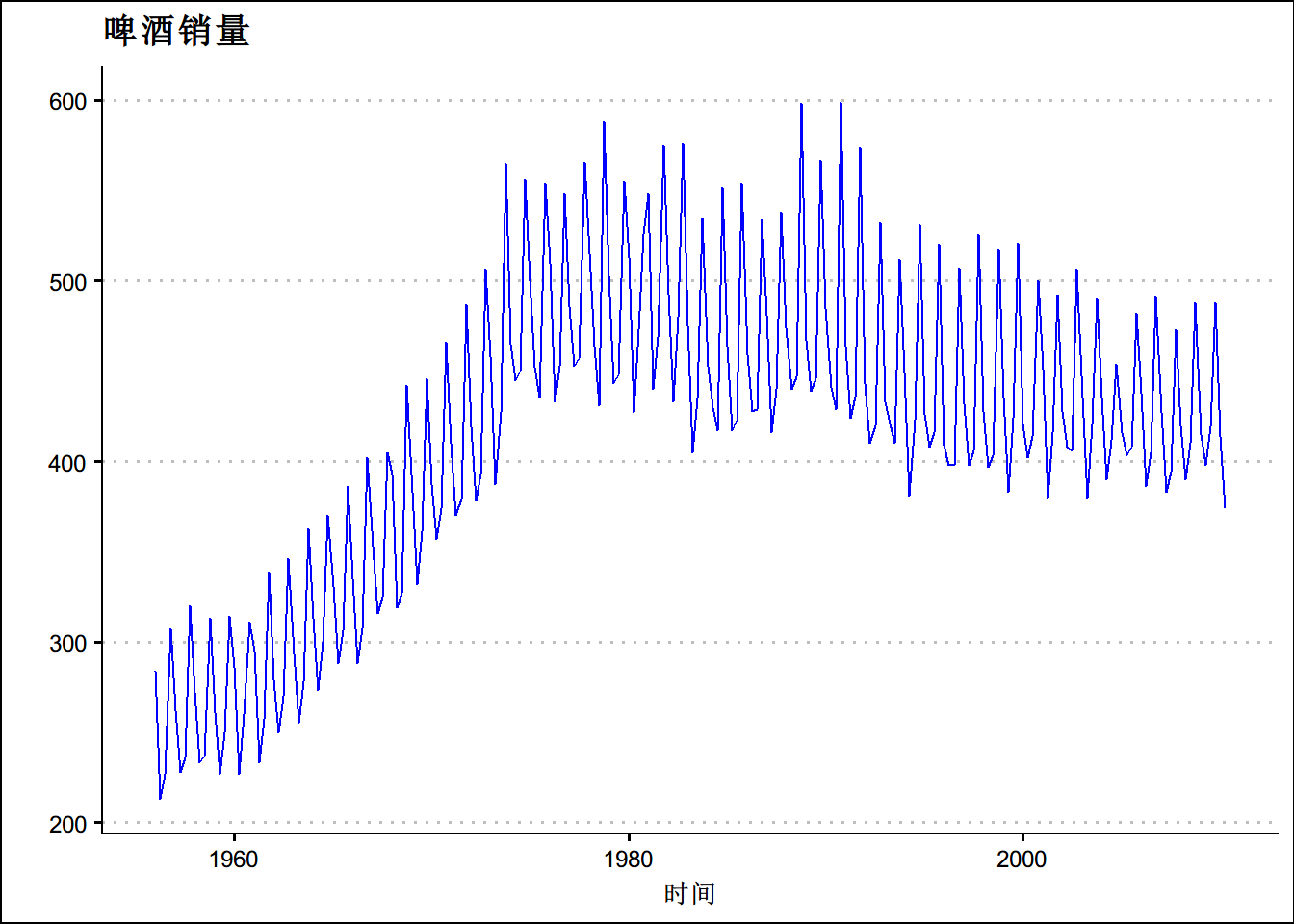
autoplot(AirPassengers,ts.colour = "red",main="乘客数量",xlab = "时间") +theme_clean()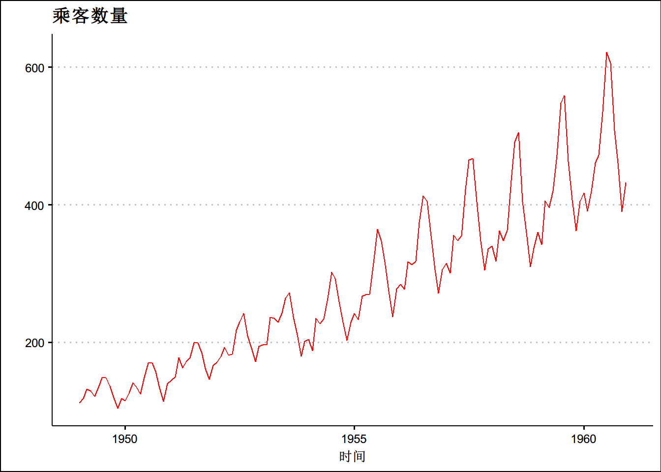
autoplot(melsyd[,"Economy.Class"]) +
  ggtitle("墨尔本 - 悉尼经济舱乘客客流量") +
  theme_clean() +
  xlab("年份") +
  ylab("千")+
  theme(text = element_text(family = "STHeiti"))+
  theme(plot.title = element_text(hjust = 0.5))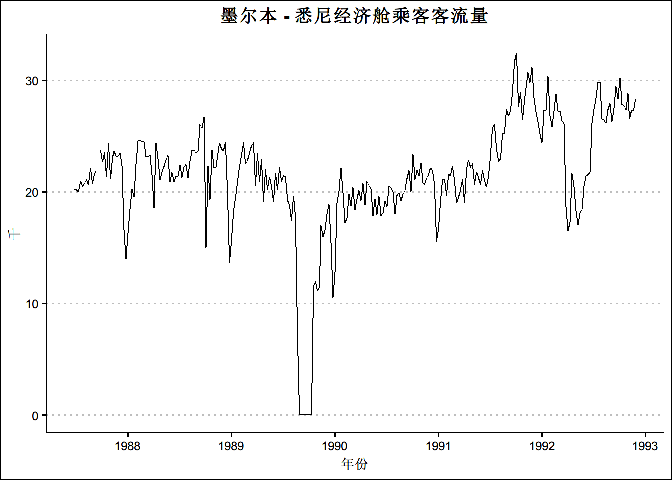
中国股市开户数的一个趋势
setwd("C:/Users/jefee/Desktop")
data <- read_csv('data2.csv')
pt<-ts(data$`信用账户新增开户投资者数:合计`,frequency=12,start=c(2011,1),end = c(2020,2))
dec_data <- decompose(pt,type='additive')
autoplot(dec_data) +theme_clean()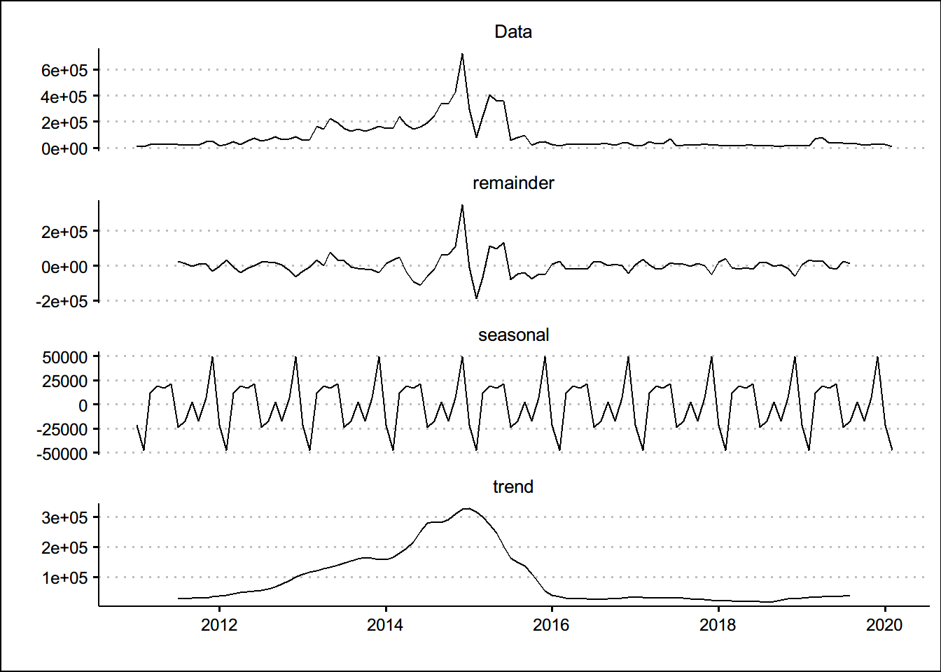
时间序列的模式
趋势
季节性
周期性
autoplot(AirPassengers )+theme_clean()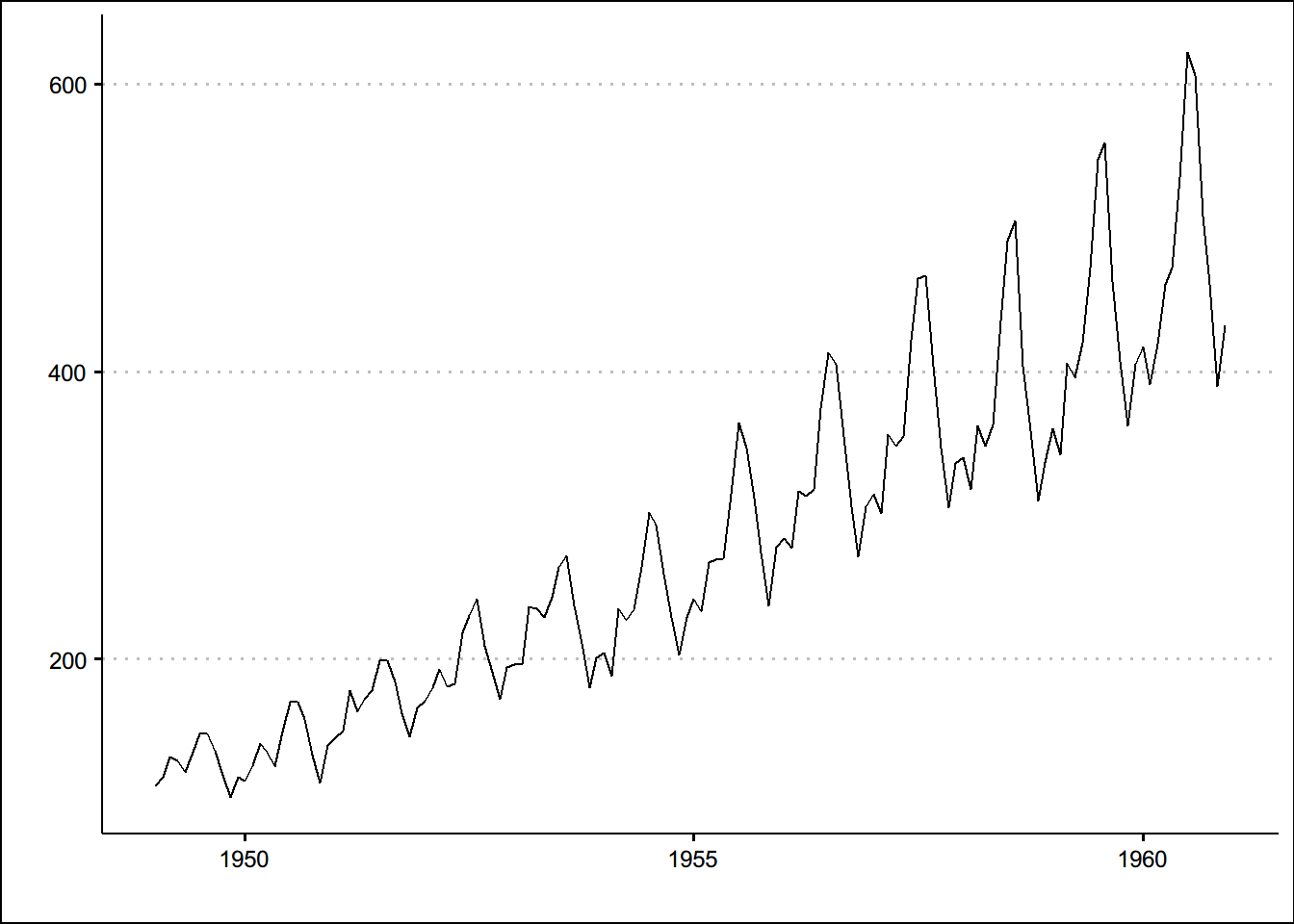
autoplot(arrivals, facets = TRUE)+theme_clean()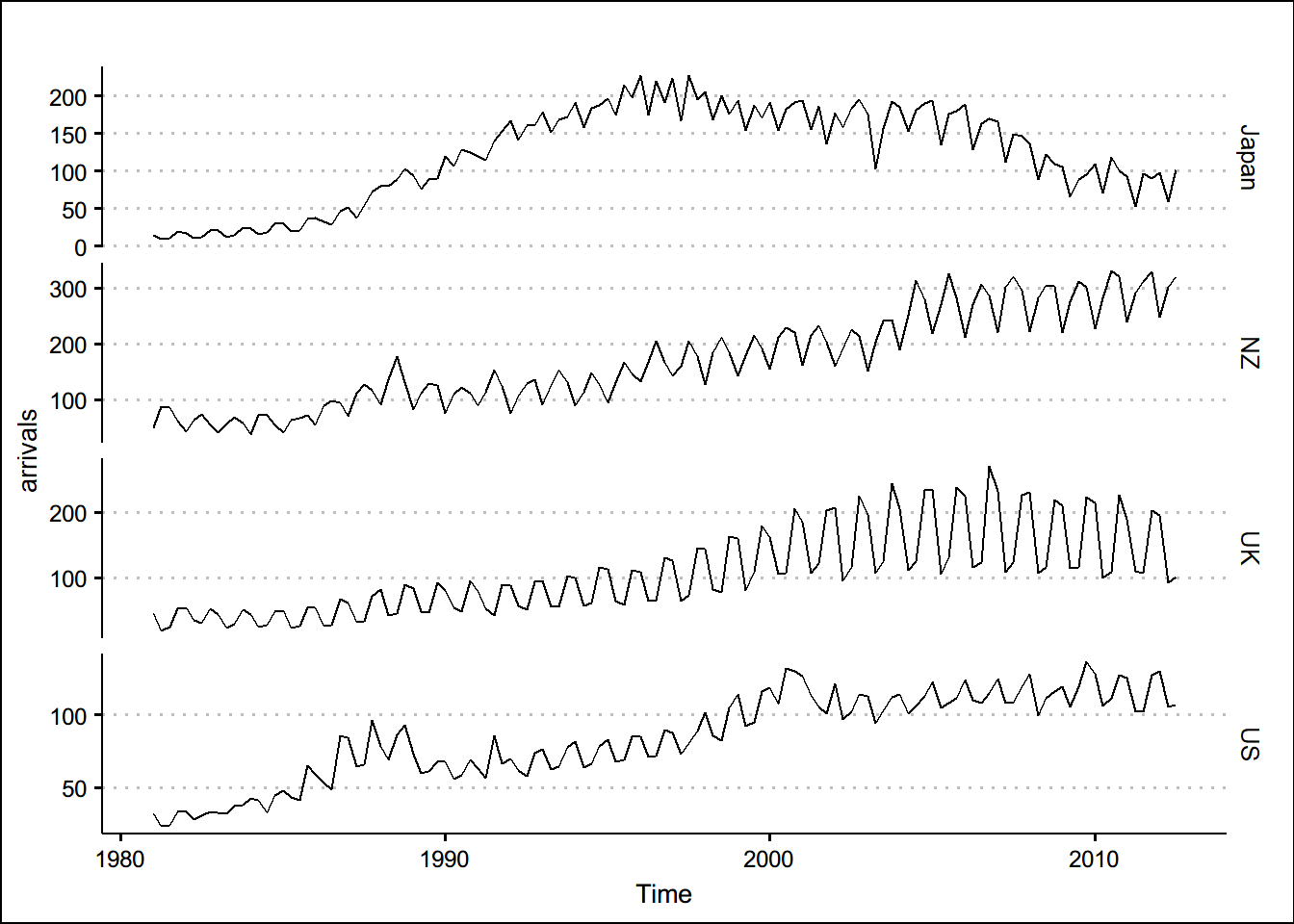
autoplot(arrivals, facets = TRUE) +
theme_clean() +
geom_smooth() +
labs(title ="到澳大利亚旅客人数",
y = "Arrivals (in thousands)",
x = NULL)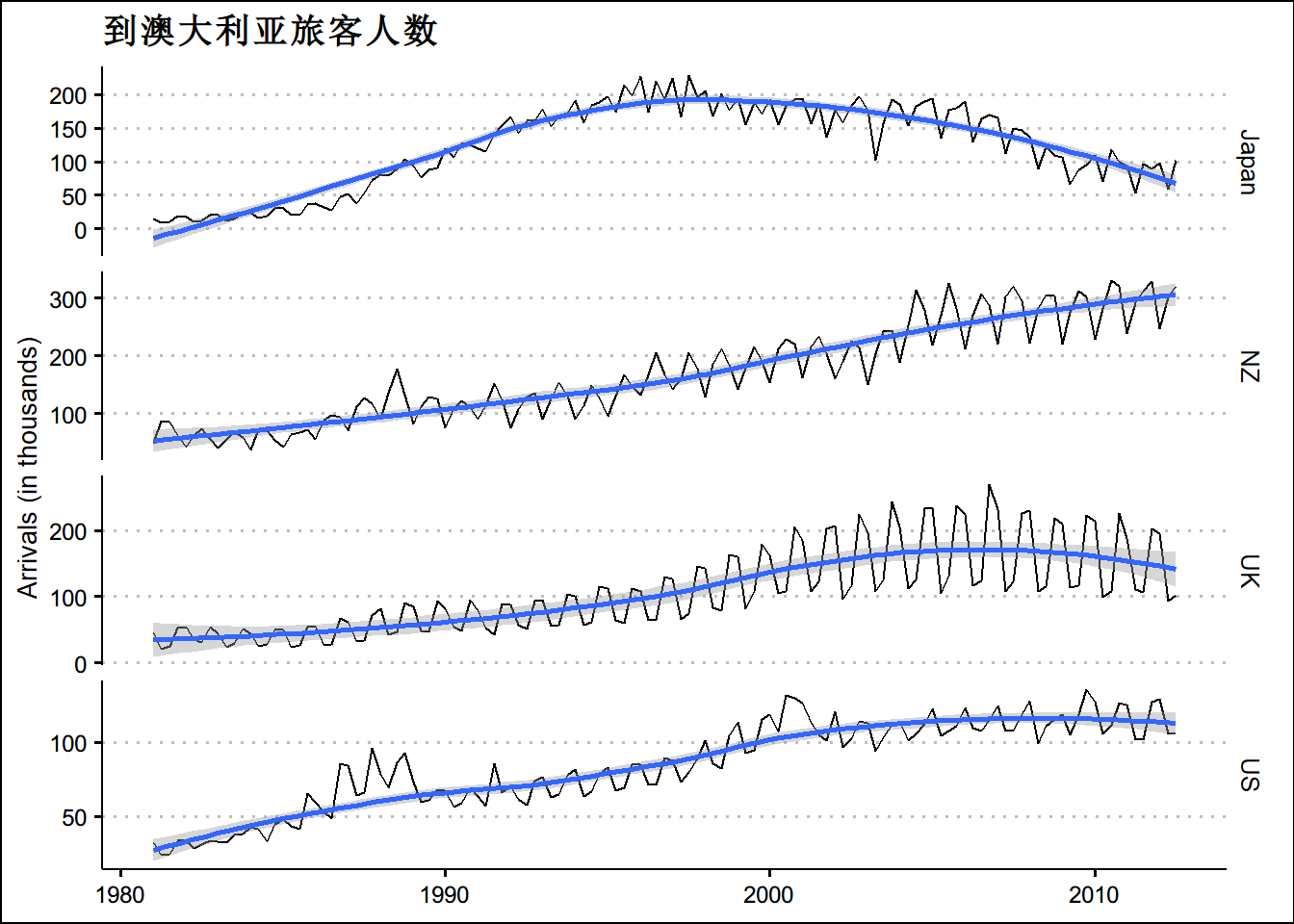 ## 季节性
ggseasonplot(a10, year.labels=TRUE, year.labels.left=TRUE) +
  xlab("月份")+
  ylab("百万(美元)") +
  ggtitle("季节图:降糖药物销量")+
  theme(text = element_text(family = "STHeiti"))+
  theme(plot.title = element_text(hjust = 0.5)) +
  theme_clean()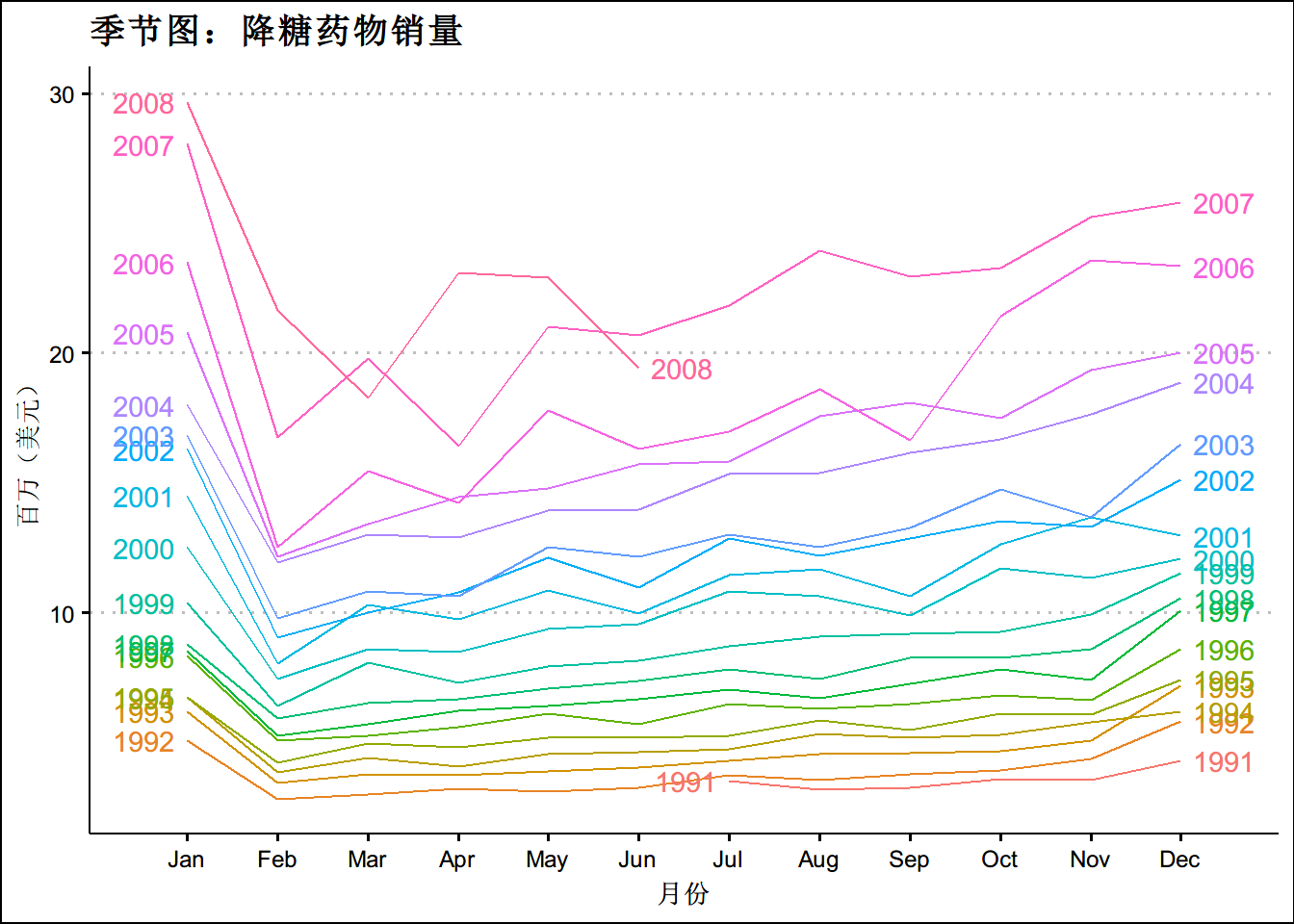
ggseasonplot(a10, polar=TRUE) +
  xlab("月份")+
  ylab("百万(美元)") +
  ggtitle("极坐标季节图:降糖药物销量")+
  theme(text = element_text(family = "STHeiti"))+
  theme(plot.title = element_text(hjust = 0.5))+
  theme_clean()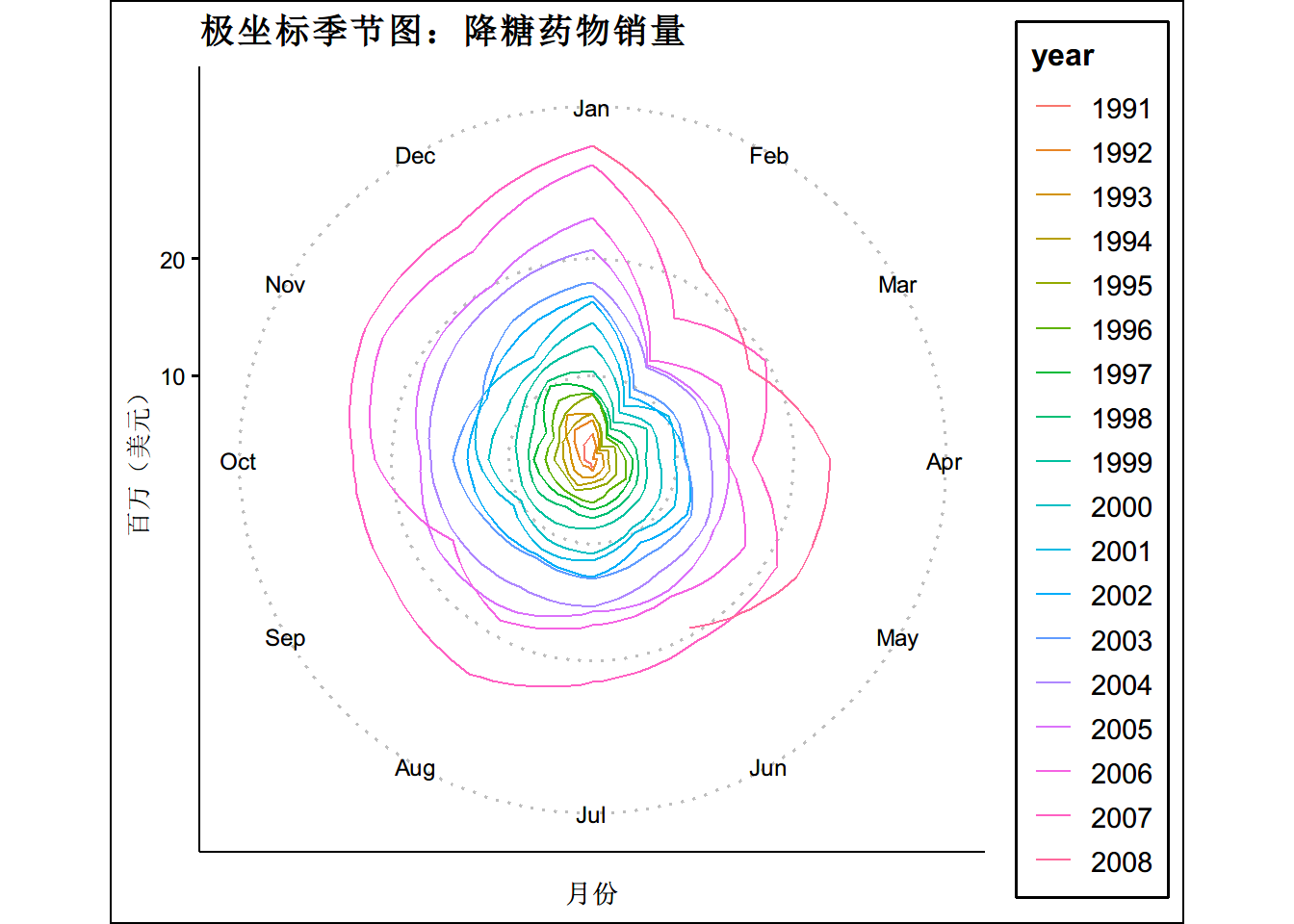
library(stats)
autoplot(stl(AirPassengers, s.window = 'periodic'), ts.colour = 'blue')+
  theme_clean()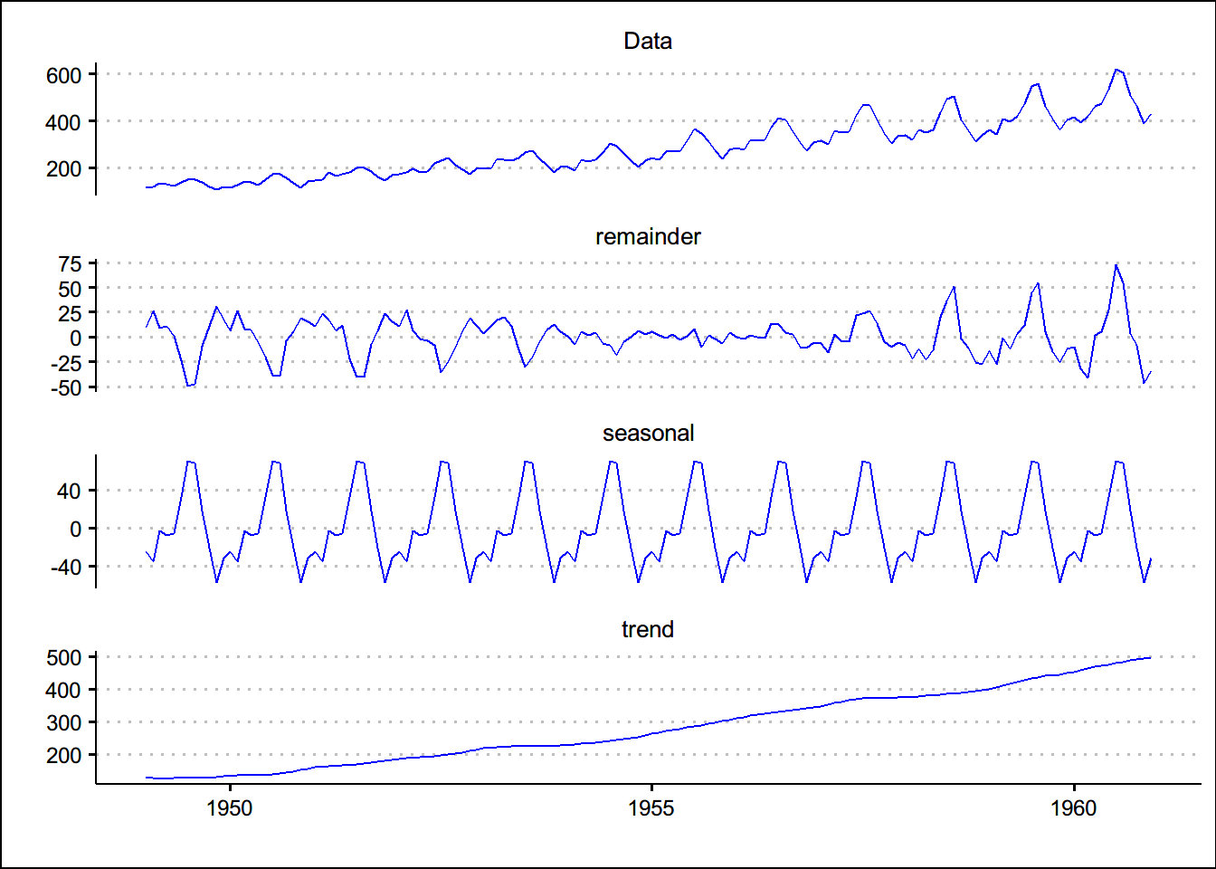
时间序列的模式
趋势
季节性
周期性
decompose_beer  <- decompose(ausbeer,type = "additive")
autoplot(decompose_beer,ts.colour = 'blue',main = "啤酒销量的加法分解")+theme_clean()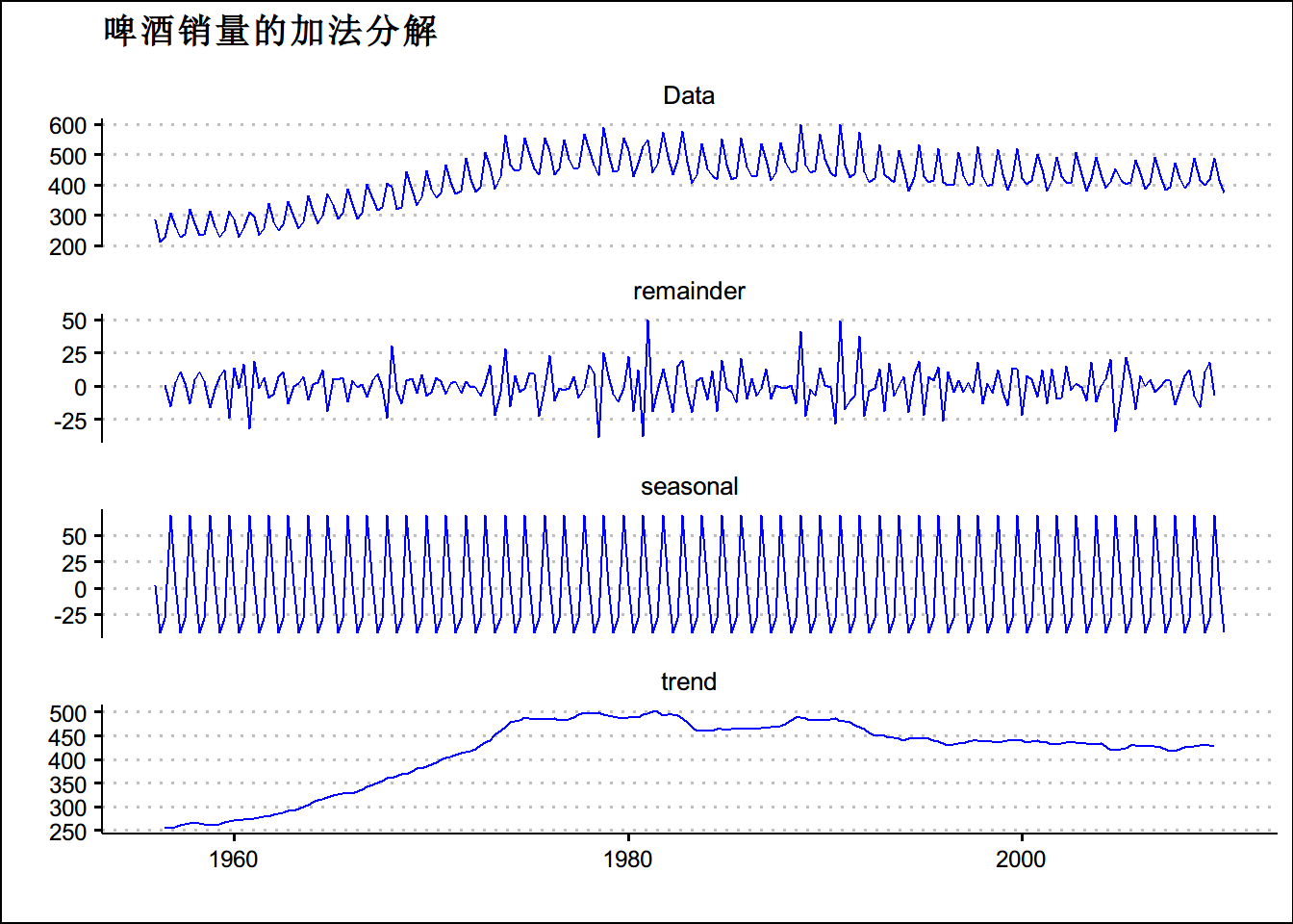
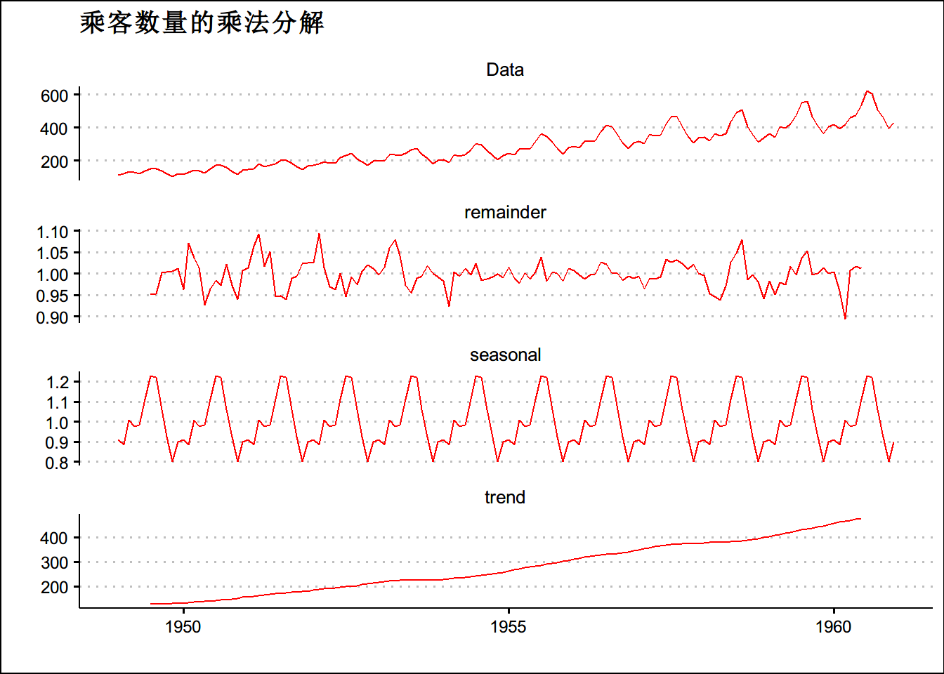
decompose_as <- decompose(AirPassengers,type= "multiplicative")
autoplot(decompose_as,ts.colour = 'red',main = "乘客数量的乘法分解")+theme_clean()